---
title: Actor Partner Interdependence Model With Multilevel Analysis
author: Mark Lai
date: "2021-10-23"
categories:
- Statistics
tags:
- multilevel
---
Every time I teach multilevel modeling (MLM) at USC, I have students interested in running the actor partner independence model (APIM) using dyadic model. While such models are easier to fit with structural equation modeling, it can also be fit using MLM. In this post I provide a software tutorial for fitting such a model using MLM, and contrast to results to SEM.
Note that this is not a conceptual introduction to APIM. Please check out [this chapter](https://psycnet.apa.org/record/2000-07611-017) and [this paper](https://psycnet.apa.org/record/2017-05295-001).
There is also [this great tutorial](https://quantdev.ssri.psu.edu/tutorials/actor-partner-interdependence-model-apim-basic-dyadicbivariate-analysis) on using the `nlme` package, which uses the dummy variable trick to allow a univariate MLM to handle multivariate analyses. The current blog post is similar but with a different package.
See also https://hydra.smith.edu/~rgarcia/workshop/Day_1-Actor-Partner_Interdependence_Model.html with the same example using `nlme::gls()`.
## Load Packages
```{r load-pkg, message = FALSE}
library(tidyverse)
library(psych)
library(glmmTMB)
```
## Data
The data set comes from https://github.com/RandiLGarcia/dyadr/tree/master/data, which has 148 married couples. You can see the codebook at https://randilgarcia.github.io/week-dyad-workshop/Acitelli%20Codebook.pdf
```{r acipair}
pair_data <- here::here("data_files", "acipair.RData")
# Download data if not already exists in local folder
if (!file.exists(pair_data)) {
  download.file("https://github.com/RandiLGarcia/dyadr/raw/master/data/acipair.RData",
                pair_data)
}
load(pair_data)
# Show data
head(acipair)
```
## Hypothetical Research Question
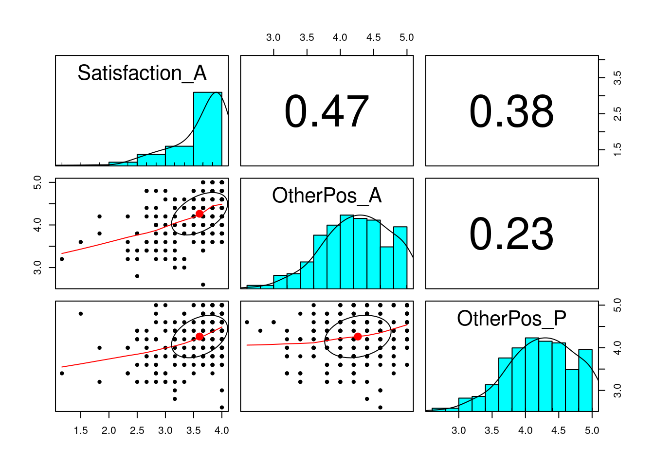
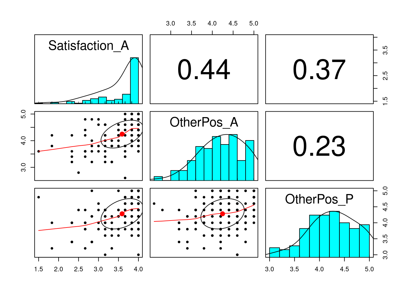
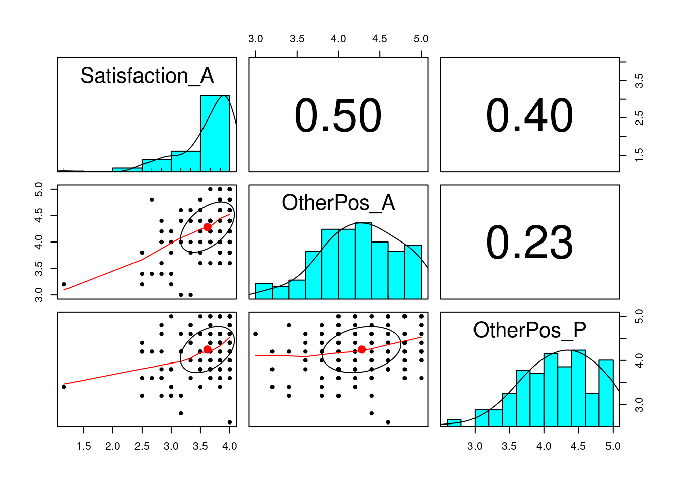
Here we have a hypothetical research question of how a person views their partners (`OtherPos_A`) and how their partner views them (`OtherPos_P`) predict their marriage satisfaction (`Satisfaction_A`).
```{r pairs-panel}
# Overall
pairs.panels(
  subset(acipair, select = c("Satisfaction_A", "OtherPos_A", "OtherPos_P"))
)
# Wife
pairs.panels(
  subset(acipair, subset = Gender_A == "Wife",
         select = c("Satisfaction_A", "OtherPos_A", "OtherPos_P"))
)
# Husband
pairs.panels(
  subset(acipair, subset = Gender_A == "Husband",
         select = c("Satisfaction_A", "OtherPos_A", "OtherPos_P"))
)
# Note the ceiling effect of satisfaction
```
In this example, there are two major paths of interest:
- Actor effect: `OtherPos_A` to `Satisfaction_A`
- Partner effect: `OtherPos_P` to `Satisfaction_A`
In addition, for *distinguishable dyads*, like husband and wives, we want the gender interactions as well, resulting in four paths of interest (actor/partner effects for husbands/wives).
# Distinguishable Dyads
Level 1:
$$
\begin{aligned}
\text{Satisfaction}_{ij} & = \beta_{0j} + \beta_{1j} \text{View Partner}_{ij} + \beta_{2j} \text{Partner View}_{ij} + \beta_{3j} \text{Gender}_{ij} \\
& \quad + \beta_{4j} \text{View Partner}_{ij} \times \text{Gender}_{ij} \\
& \quad + \beta_{5j} \text{Partner View}_{ij} \times \text{Gender}_{ij} + e_{ij} \\
e_{ij} & \sim N(0, \sigma^2_{ij}) \\
\log(\sigma^2_{ij}) & = \beta^{s}_{0j} + \beta^{s}_{1j} \text{Gender}_{ij}
\end{aligned}
$$
Level 2:
$$
\begin{aligned}
\beta_{0j} & = \gamma_{00} + u_{0j} \\
\beta_{1j} & = \gamma_{10} \\
\beta_{2j} & = \gamma_{20} \\
\beta_{3j} & = \gamma_{30} \\
\beta_{4j} & = \gamma_{40} \\
\beta_{5j} & = \gamma_{50} \\
\beta^{s}_{0j} & = \gamma^{s}_{00} \\
\beta^{s}_{1j} & = \gamma^{s}_{10} \\
u_{0j} | \text{Wife} & \sim N(0, \tau^2_{0 | H}) \\
u_{1j} | \text{Husband} & \sim N(0, \tau^2_{0 | W})
\end{aligned}
$$
Note that the variance components are allowed to be different across genders.
```{r m_apim}
m_apim <- glmmTMB(
  Satisfaction_A ~ (OtherPos_A + OtherPos_P) * Gender_A +
    us(0 + Gender_A | CoupleID),
  dispformula = ~ Gender_A,
  data = acipair,
  REML = FALSE
)
summary(m_apim)
```
The model results show:
- Actor effect for Wife: 0.37 (SE = 0.07)
- Partner effect for Wife: 0.32 (SE = 0.08)
- Difference of actor effect (Husband - Wife): 0.05 (SE = 0.10)
- Difference of partner effect (Husband - Wife): -0.06 (SE = 0.11)
- Gender difference (Husband - Wife) when Partner View is 0: 0.08 (SE = 0.39)
We can also estimate the actor and partner effects for both Husband and Wife by suppressing the intercept:
```{r m_apim2}
m_apim2 <- glmmTMB(
  Satisfaction_A ~ 0 + Gender_A + (OtherPos_A + OtherPos_P):Gender_A +
    us(0 + Gender_A | CoupleID),
  dispformula = ~ Gender_A,
  data = acipair,
  REML = FALSE,
  # The default optimizer did not converge; try optim
  control = glmmTMBControl(
    optimizer = optim,
    optArgs = list(method = "BFGS")
  )
)
summary(m_apim2)
```
# Indistinguishable Dyads
As the interaction terms were not significant, one may want to remove them. Similarly, the variance components did not look too different across genders, so we may make them equal as well:
```{r m2}
m2 <- glmmTMB(
  Satisfaction_A ~ Gender_A + OtherPos_A + OtherPos_P + (1 | CoupleID),
  dispformula = ~ 1,
  data = acipair,
  REML = FALSE
)
summary(m2)
```
Finally, we may also remove the main effect for Gender:
```{r m3}
m3 <- glmmTMB(
  Satisfaction_A ~ OtherPos_A + OtherPos_P + (1 | CoupleID),
  dispformula = ~ 1,
  data = acipair,
  REML = FALSE
)
summary(m3)
```
## Model Comparison
```{r anova-m1-2-3}
anova(m_apim, m2, m3)
```
There model with all paths equal is the best in terms of AIC and BIC, and the likelihood ratio tests were not significant.
## Using SEM
## Distinguishable Dyads
```{r apim_fit}
# Wide format
aciwide <- filter(acipair, Partnum == 1)  # Actor = Wife; Partner = Husband
library(lavaan)
apim_mod <- ' Satisfaction_A + Satisfaction_P ~ OtherPos_A + OtherPos_P '
apim_fit <- sem(apim_mod, data = aciwide)
summary(apim_fit)
```
```{r plot-apim-fit, fig.show = "hide"}
library(semPlot)
library(semptools)
p1 <- semPaths(apim_fit, what = "est",
               rotation = 2,
               sizeMan = 15,
               nCharNodes = 0,
               edge.label.cex = 1.15,
               label.cex = 1.25)
```
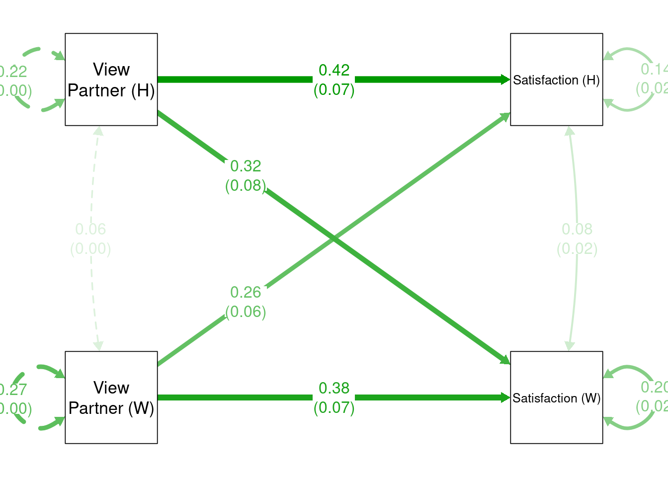
```{r plot-apim-fit-2}
my_label_list <- list(list(node = "Satisfaction_A", to = "Satisfaction (W)"),
                      list(node = "Satisfaction_P", to = "Satisfaction (H)"),
                      list(node = "OtherPos_A", to = "View\nPartner (W)"),
                      list(node = "OtherPos_P", to = "View\nPartner (H)"))
p2 <- change_node_label(p1, my_label_list)
p3 <- mark_se(p2, apim_fit, sep = "\n")
my_position_list <- c("Satisfaction_A ~ OtherPos_P" = .25,
                      "Satisfaction_P ~ OtherPos_A" = .25)
p4 <- set_edge_label_position(p3, my_position_list)
plot(p4)
```
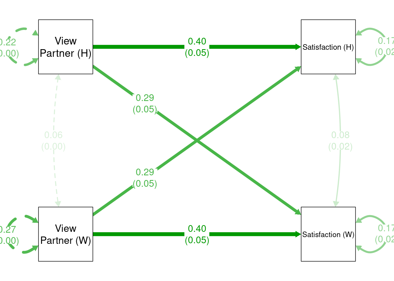
## Indistinguishable Dyads
```{r apim2_fit}
apim2_mod <- ' Satisfaction_A ~ a * OtherPos_A + p * OtherPos_P
               Satisfaction_P ~ p * OtherPos_A + a * OtherPos_P
               # Constrain the variances and means to be equal
               Satisfaction_A ~~ v * Satisfaction_A
               Satisfaction_P ~~ v * Satisfaction_P
               Satisfaction_A ~ m * 1
               Satisfaction_P ~ m * 1 '
apim2_fit <- sem(apim2_mod, data = aciwide)
summary(apim2_fit)
```
```{r plot-apim-fit-3, fig.show = "hide"}
p1 <- semPaths(apim2_fit, what = "est",
               rotation = 2,
               sizeMan = 15,
               nCharNodes = 0,
               edge.label.cex = 1.15,
               label.cex = 1.25,
               intercepts = FALSE)
```
```{r plot-apim-fit-4}
my_label_list <- list(list(node = "Satisfaction_A", to = "Satisfaction (W)"),
                      list(node = "Satisfaction_P", to = "Satisfaction (H)"),
                      list(node = "OtherPos_A", to = "View\nPartner (W)"),
                      list(node = "OtherPos_P", to = "View\nPartner (H)"))
p2 <- change_node_label(p1, my_label_list)
p3 <- mark_se(p2, apim2_fit, sep = "\n")
my_position_list <- c("Satisfaction_A ~ OtherPos_P" = .25,
                      "Satisfaction_P ~ OtherPos_A" = .25)
p4 <- set_edge_label_position(p3, my_position_list)
plot(p4)
```
The results are basically identical.