---
title: Confidence Intervals for Multilevel Mediation
author: Mark Lai
date: "2017-08-25"
bibliography: references.bib
draft: no
categories:
- Statistics
tags:
- R
- multilevel
- mediation
- confidence interval
- Bayesian
---
```{r setup, include=FALSE}
knitr::opts_chunk$set(echo = TRUE, message = FALSE)
comma <- function(x) format(x, digits = 2, big.mark = ",")
```
The data are from the `mediation` package, which are simulated data with the
source of the Education Longitudinal Study of 2002. For the interest of time as
well as to consider situations where asymptotic normality may not hold, I only
select 50 schools (out of 568) from the sample.
```{r}
library(tidyverse)
library(lme4)
library(mediation)
data("school", package = "mediation")
# Select only a random sample of 24 schools, stratified by
# `coed` and `catholic`
set.seed(827)
# School-level subsample:
school_sub <- school %>% sample_n(size = 50) %>% arrange(SCH_ID)
school_sub %>% as_data_frame()
# Student-level subsample:
student_sub <- student %>% filter(SCH_ID %in% school_sub$SCH_ID)
student_sub %>% as_data_frame()
```
The example is taken from [the vignette of the `mediation`
package](ftp://ftp.gr.vim.org/mirrors/CRAN/web/packages/mediation/vignettes/mediation.pdf)
(p. 19), where a school-level poverty indicator (`free`, "percent of 10th grade
students receiving free lunch" with 7 levels) is hypothesized to cause
school-level morale (`smorale` with 4 levels), which in turn causes
student-level tardiness (`late`, "frequency in which the student was late for
school" with 5 levels). For the mediator equation, the school-level covariates
are `catholic` and `coed`; for the outcome equation, in addition to the
school-level covariates, student-level covariates are `gender`, `income`,
`pared`.
## Quasi-Bayesian/Monte Carlo CI With the `mediation` Package
The `mediate()` function provides CI for the indirect effect using
Quasi-Bayesian method, which I believe is similar to the Monte Carlo method by
assuming normality of the $a$ path and the $b$ path. Bootstrapping is not
supported when one equation is a multilevel model.
```{r}
# Using the mediation package
# 1. Mediator equation
med_fit <- lm(smorale ~ free + catholic + coed, data = school_sub)
# 2. Outcome equation
out_fit <- lmer(late ~ free + smorale + catholic + coed +
                  gender + income + pared + (1 | SCH_ID), data = student_sub)
# Record the time:
system.time(med_out <- mediate(med_fit, out_fit, treat = "free",
                               mediator = "smorale",
                               control.value = 3, treat.value = 4, sims = 500))
summary(med_out) # Summary of mediation analysis
```
The output gives the "ACME" (average causal mediation effect) estimate, which
equals estimator of $ab$ under a normal model, as well as "ADE" (average direct
effect), which equals estimator of $c'$ under a normal model, and ACME and ADE
add up to the "Total Effect", and the proportion mediated as estimating $ab /
(ab + c')$. The posterior median was used for all the quantities, together
with the credible intervals.
One can use the posterior samples (e.g., `d0.sim` for the posterior samples of
the $a$ path) to compute any derived quantities. However, the posterior samples
for the variance components are not available, so one cannot compute
standardized coefficients or effect sizes defined using variance components.
## Analytical Approaches for CI With the `RMediation` Package
The two main analytical approaches are [see @MacKinnon2004]:
1. distribution of product of coefficients
2. Asymptotic normal CI (or Wald CI)
### Distribution of Product of Coefficients
This approach uses the quantiles of the distribution of $ab$ when $a$ and $b$
are assumed bivariate normal. Therefore, the Quasi-Bayesian/Monte Carlo
approach can be viewed as an approximation of it. It is, however, less flexible
as it does not provide distributions of other derived quantities (e.g.,
proportion mediated).
```{r}
# With RMediation
nmtx <- "free"  # name of treatment variable
nmmed <- "smorale"  # name of mediator
a <- coef(med_fit)[nmtx]  # estimate of a path with name removed
va <- vcov(med_fit)[nmtx, nmtx]  # sampling variance of a path
b <- fixef(out_fit)[nmmed]  # estimate of b path with name removed
vb <- vcov(out_fit)[nmmed, nmmed]  # sampling variance of b path
# Distribution of Product of Coefficients
(med_dop <- RMediation::medci(mu.x = a, mu.y = b, type = "dop",
                              se.x = sqrt(va), se.y = sqrt(vb)))
```
### Asymptotic Normal CI
\newcommand{\SE}{\textit{SE}}
The asymptotic *SE* for the product of two normal variables, as defined
in the `RMediation` package, is:
$$\SE(\hat a \hat b) = \sqrt{a^2 \SE^2(b) + b^2 \SE^2(a) +
2 ab \SE(a) \SE(b) r_{\hat a \hat b} +
\SE^2(a) \SE^2(b) r_{\hat a \hat b}}$$
And we replace $a$, $b$, $\SE(a)$, $\SE(b)$ with the corresponding sample
estimates. Note that as we use separate equations to obtain $\hat a$ and
$\hat b$, the correlation between them, $r_{\hat a \hat b}$, is assumed zero,
so the asymptotic *SE* is computed as:
$$\SE(\hat a \hat b) = \sqrt{a^2 \SE^2(b) + b^2 \SE^2(a)}$$
and the Asymptotic symmetric CI is $\hat a \hat b \pm 1.96 \SE(\hat a \hat b)$.
```{r}
# Assuming Asymptotic Normality
(med_asym <- RMediation::medci(mu.x = a, mu.y = b, type = "asymp",
                               se.x = sqrt(va), se.y = sqrt(vb)))
```
## Case Bootstrap
All the above approaches involve normality assumptions: the quasi-Bayesian and
the distribution of product approaches assume the sampling distribution of $\hat
a$ and $\hat b$ are jointly normal, whereas the asymptotic CI assumes that the
sampling distribution of $\hat a \hat b$ is normal. In small sample and/or with
non-normal data, such assumptions may not hold. That is one of the reasons that
resampling methods, in particular the bootstrap, is popular for single-level
mediation analysis.
There are many methods to do bootstrapping with multilevel analysis [see
@VanderLeeden2008 for an overview]. However, to my knowledge most of them are
not directly built in multilevel software, especially for mediation models. A
relatively simple bootstrapping method is the *case bootstrap*, which resample
intact clusters with replacement. The advantage is that it basically makes no
assumption about the data, such as the specification of the functional form and
the distribution of the random effects. Therefore the results should be robust.
The drawback, however, is that when the cluster sizes are not balanced, as in
our example, it results in bootstrap samples with different level-1 sample
sizes. And based on my experience it is generally less efficient and requires a
relatively large number of clusters to perform well. Below is my implementation
of the case bootstrap for this example, which include the indirect effect and
some derived quantities.
```{r}
library(boot)  # load the boot package
# Get the unique school IDs as a global variable
sch_id <- school_sub$SCH_ID

lv1_resample <- function(new_lv2_id, data = student_sub,
                         group_var = "SCH_ID") {
  # Return a resampled lv-1 data set given an input of cluster values
  #
  # Args:
  #   new_lv2_id: A vector (character/numeric) showing the cluster values
  #               to be selected.
  #   data: The lv-1 data set to be resampled.
  #   group_var: A character vector of length 1 indicating the variable name
  #              for cluster ID
  # Returns:
  #   A data.frame object with the resampled data.
  group <- data[[group_var]]
  N <- nrow(data)
  new_lv1_index <- unlist(
    lapply(new_lv2_id, function(i) seq_len(N)[group == i]))
  gp_tab <- table(group, dnn = NULL)
  gp_length <- gp_tab[as.character(new_lv2_id)]
  # `new_group` make sure that each resampled cluster get a distinct
  # cluster ID.
  new_group <- rep(seq_along(new_lv2_id), gp_length)
  new_data <- data[new_lv1_index, , drop = FALSE]
  new_data[group_var] <- new_group
  rownames(new_data) <- NULL
  new_data
}

ab_resample <- function(data_lv2, i, ...) {
  new_sch_id <- sch_id[i]
  med_fit <- lm(smorale ~ free + catholic + coed, data = data_lv2[i, ])
  new_stud_dat <- lv1_resample(new_sch_id, ...)
  # Use `calc.dervis` to skip computing the derivatives and save
  # some time for each bootstrap replication
  out_fit <- lmer(late ~ free + smorale + catholic + coed +
                  gender + income + pared + (1 | SCH_ID), data = new_stud_dat,
                  control = lmerControl(calc.derivs = FALSE))
  a <- unname(coef(med_fit)[nmtx])
  b <- unname(fixef(out_fit)[nmmed])
  ab <- a * b
  va <- vcov(med_fit)[nmtx, nmtx]
  vb <- vcov(out_fit)[nmmed, nmmed]
  # variance components (for standardizing y):
  sigma_y <- sigma(out_fit)  # level-1 SD
  tau <- getME(out_fit, "theta") * sigma_y  # random intercept SD
  # c-prime (for getting proportion mediated)
  c_prime <- unname(fixef(out_fit)[nmtx])
  c(ab = ab,
    vab = a^2 * vb + b^2 * va,
    ab_stdy = ab / sqrt(tau^2 + sigma_y^2),
    pm = ab / (ab + c_prime))
}
```
```{r}
system.time(med_boo <- boot(school_sub, ab_resample, 1000))
med_boo
```
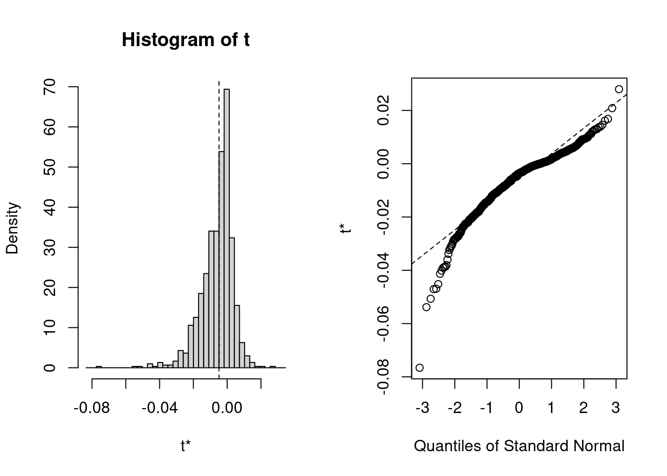
We can plot the bootstrap distributions (Note the non-normality)
```{r}
plot(med_boo, index = 1L)
```
The output shows that the indirect effect estimate was biased by
`r comma((mean(med_boo$t[ , 1]) / med_boo$t0["ab"] - 1) * 100)`%, whereas the
estimated sampling variance was biased by
`r comma((mean(med_boo$t[ , 2]) / med_boo$t0["vab"] - 1) * 100)`%! (or
`r comma((mean(sqrt(med_boo$t[ , 2])) / sqrt(med_boo$t0["vab"]) - 1) * 100)`%
for standard error bias)
### Bootstrap CI
#### Indirect effect
Generally BCa (bias-corrected and accelerated) and studentized CIs (also called
bootstrap-$t$) are more accurate [see @Davison1997, @VanderLeeden2008,
@Cheung2008]. However, the BCa needs the accerlation value (which is used to
correct for skewness), which is estimated using the regression estimation here,
and to my knowledge its use for multilevel data has not been tested.
The studentized CI requires the use of the sampling variance of the statistic to
be bootstrapped, which is why I also computed the asymptotic variance of
the indirect effect in each bootstrap replication.
```{r}
# For (unstandardized) indirect effect
(med_bootci <- boot.ci(med_boo, type = "all", index = 1:2))
```
As you can see, for the indirect effect estimate, both BCa and studentized CIs
gave results that are closer compared to other types of CIs. The BCa was known
to sometimes overcorrect for skewness, and in this case it might seem to be
pushing the confidence limits to the right.
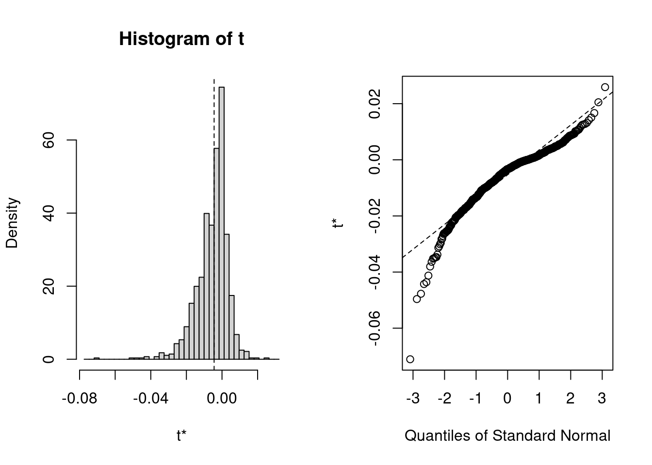
#### $y$-standardized indirect effect
We also can get study the the indirect effect with $y$ standardized, referred to
as $ab_{ps}$ in the literature, defined as
$$ab_{ps} = \frac{ab}{\sqrt{\tau^2_y + \sigma^2_y}},$$
where $\tau^2_y + \sigma^2_y$ is the total variance of $y$. $ab_{ps}$ has the
interpretation of:
> Every unit increase in $x$ (treatment variable) results in a change of
$ab_{ps}$ standard deviations in $y$ through the mediator.
First look at the bootstrap distribution:
```{r}
plot(med_boo, index = 3L)
```
It's easy to get the bootstrap CIs. However, for the $y$-standardized indirect
effect and the proportion mediated it would be more work to obtain the sampling
variance estimates (which can be obtained with the delta method or with other
resampling method within each bootstrap sample; the former needs some derivation
and may not be very accurate and the latter will increase the computation time
by a factor of 100 or more, which is not practical), so I did not request for
the studentized CI.
```{r}
# For y-standardized indirect
boot.ci(med_boo, type = c("norm", "basic", "perc", "bca"), index = 3L)
```
As shown in the result, BCa interval is wider but with higher lower and upper
confidence limits. For single-level mediation @Cheung2009 showed that the
percentile and BCa CIs are better than Wald CI and using the `PRODCLIN CI`
macro. It is still an open question how the different bootstrap CIs perform
in multilevel mediation.
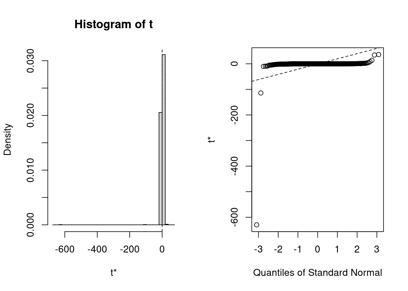
#### Proportion mediated
Again, check the bootstrap distribution:
```{r}
plot(med_boo, index = 4L)
```
Finally, we can get CIs for proportion mediated:
```{r}
# For proportion mediated
boot.ci(med_boo, type = c("norm", "basic", "perc", "bca"), index = 4L)
```
The percentile CI (and to a less degree the basic CI) was close to the one given
with the `mediation` package, whereas the normal bootstrap CI and the BCa CI had
much wider intervals. After all, I don't think proportion mediated would be a
good measure of effect size, as also pointed out in @Miocevic2017.
Note that I only illustrated case bootstrap in this post. For clustered data,
in @Davison1997, it was found that residual bootstrap may result in better
coverage. I may implement residual bootstrap for mediation in the R package
I am working on, `bootmlm`.
## Fully Bayesian Approach With `rstan`
Brad Efron said the bootstrap can be an approximation of Bayesian estimation. So
we can actually do a fully Bayesian model, which actually is not complicated to
fit. It is basically putting a Bayesian multiple regression and a random
intercept model together. Given that the scales of the variables are quite
similar and generally with SD = 0.5 to 2, I used weakly informative priors with
$N(0, 10^2)$ for the fixed effects and $t_3(0, 10^2)$ for the random effect
standard deviations (i.e., $\sigma_m$, $\tau_y$, $\sigma_y$).
The Bayesian model here assumes normality in the random effects but not
asymptotic normality of the posterior distributions of $a$ and $b$ and other
parameters.
```{r}
library(rstan)
rstan_options(auto_write = TRUE)
options(mc.cores = 2L)
library(coda)
```
Below is the STAN code for the multilevel mediation model:
```{r, echo=FALSE, comment=NA}
cat(readLines("stan_mlm_mediate.stan"), sep = '\n')
```
```{r, results='hide'}
numeric_id <- function(id) {
  # Make group ID to be natural numbers from 1, 2, ..., as needed in the
  # STAN program
  match(id, unique(id))
}
med_sdata <- list(J = nrow(school_sub),
                  M = school_sub$smorale,
                  Kw = 4,
                  W = cbind(1, school_sub[c("free", "catholic", "coed")]),
                  N = nrow(student_sub),
                  Y = student_sub$late,
                  Kx = 8,
                  X = cbind(1, student_sub[c("free", "smorale", "catholic",
                                             "coed", "gender", "income",
                                             "pared")]),
                  gid = numeric_id(student_sub$SCH_ID))
med_stan <- stan("stan_mlm_mediate.stan", data = med_sdata,
                 pars = c("temp_b0_m", "temp_b0_y", "a", "b",
                          "sigma_m", "sigma_y", "tau_y",
                          "ab", "ab_stdy", "pm"))
```
### Posterior (Credible) Intervals
We can get the commonly-used equal-tailed interval or the shorter (but maybe
less stable) highest posterior density interval (HPDI).
```{r, fig.height=3, fig.width=3, out.width="50%"}
# Extract the posterior samples
pars_post <- as.matrix(med_stan, pars = c("ab", "ab_stdy", "pm"))
# Posterior distribution of ab:
hist(pars_post[ , 1], xlab = "ab", main = "Posterior distribution of ab")
# Equal-tailed interval:
(post_ci <- apply(pars_post, 2, quantile, probs = c(.025, .975)))
# HPDI
(post_hpdi <- coda::HPDinterval(as.mcmc(pars_post)))
```
## Summary Table of Different CIs:
```{r}
format_ci <- function(ci) {
  paste0("(", paste(comma(ci), collapse = ","), ")")
}
data_frame(Method = c("Quasi-Bayesian", "DOP", "Asymptotic",
                      "Boot Studentized", "Boot Percentile",
                      "Boot BCa", "Bayesian CI", "Bayesian HPDI"),
           `95% CI` = c(format_ci(med_out$d0.ci),
                        format_ci(med_dop[[1]]),
                        format_ci(med_asym[[1]]),
                        format_ci(tail(med_bootci$student[1, ], 2L)),
                        format_ci(tail(med_bootci$percent[1, ], 2L)),
                        format_ci(tail(med_bootci$bca[1, ], 2L)),
                        format_ci(post_ci[ , "ab"]),
                        format_ci(post_hpdi["ab", ]))) %>%
  knitr::kable()
```
The CIs across methods are somewhat similar, with the exception of BCa and
studentized bootstrap CIs and the asymptotic CI, with the two bootstrap CIs
having wider intervals. Further studies are needed to compare their performance.
## Bibliography