library(tidyverse)
library(haven)
library(lme4)
library(brms)
library(rstan)
# rstan_options(auto_write = TRUE)
# options(mc.cores = 2L)Bayesian MLM With Group Mean Centering
Statistics
This post is re-rendered on 2024-03-21 with cleaner and more efficient STAN code.
In the past week I was teaching a one-and-a-half-day workshop on multilevel modeling (MLM) at UC, where I discussed the use of group mean centering to decompose level-1 and level-2 effects of a predictor. In that session I ended by noting alternative approaches that reduce bias (mainly from Lüdtke et al. 2008). That lead me also consider the use of Bayesian methods for group mean centering, which will be demonstrated in this post. (Turns out Zitzmann, Lüdtke, and Robitzsch 2015 has already discussed something similar, but still a good exercise.)
The Problem
In some social scienc research, a predictor can have different meanings at different levels. For example, student’s competence, when aggregated to the school level, becomes the competitiveness of a school. As explained in the big-fish-little-pond effect, whereas the former can help an individual’s self-concept, being in a more competitive environment can hurt one’s self-concept. Traditionally, and still popular nowadays, we investigate the differential effects of a predictor, \(X_{ij}\), on an outcome at different levels by including the group means, \(\bar X_{.j}\), in the equation.
The problem, however, is that unless each cluster (e.g., school) has a very large sample size, the group means will not be very reliable. This is true even when the measurement of \(X_{ij}\) is perfectly reliable. This is not difficult to understand: just remember in intro stats we learn that the standard error of the sample mean is \(\sigma / \sqrt{N}\), so with limited \(N\) our sample (group) mean can be quite different from the population (group) mean.
What’s the problem when the group means are not reliable? Regression literature has shown that unreliability in the predictors lead to downwardly biased coefficients, which is what happen here. The way to account for that, in general, is to treat the unreliable as a latent variable, which is the approach discussed in Lüdtke et al. (2008) and also demonstrated later in this post.
Demonstration
Let’s compare the results using the well-known High School and Beyond Survey subsample discussed in the textbook by Raudenbush and Bryk (2002). To illustrate the issue with unreliability of group means, I’ll use a subset of 800 cases, with a random sample of 5 cases from each school.
hsb <- haven::read_sas('https://stats.idre.ucla.edu/wp-content/uploads/2016/02/hsb.sas7bdat')
# Select a subsample
set.seed(123)
hsb_sub <- hsb %>% group_by(ID) %>% sample_n(5)
hsb_sub
# A tibble: 800 × 12
# Groups: ID [160]
ID SIZE SECTOR PRACAD DISCLIM HIMINTY MEANSES MINORITY FEMALE SES
<chr> <dbl> <dbl> <dbl> <dbl> <dbl> <dbl> <dbl> <dbl> <dbl>
1 1224 842 0 0.35 1.60 0 -0.428 0 1 -0.478
2 1224 842 0 0.35 1.60 0 -0.428 0 0 0.332
3 1224 842 0 0.35 1.60 0 -0.428 0 1 -0.988
4 1224 842 0 0.35 1.60 0 -0.428 0 0 -0.528
5 1224 842 0 0.35 1.60 0 -0.428 0 1 -1.07
6 1288 1855 0 0.27 0.174 0 0.128 0 1 0.692
7 1288 1855 0 0.27 0.174 0 0.128 0 0 -0.118
8 1288 1855 0 0.27 0.174 0 0.128 0 0 1.26
9 1288 1855 0 0.27 0.174 0 0.128 1 1 -1.47
10 1288 1855 0 0.27 0.174 0 0.128 0 0 0.222
# ℹ 790 more rows
# ℹ 2 more variables: MATHACH <dbl>, `_MERGE` <dbl>With the subsample, let’s study the association of socioeconomic status (SES) with math achievement (MATHACH) at the student level and the school level. The conventional way is to do group mean centering of SES, by computing the group means and the deviation of each SES score from the corresponding group mean.
hsb_sub <- hsb_sub %>% ungroup() %>%
  mutate(SES_gpm = ave(SES, ID), SES_gpc = SES - SES_gpm)
To make things simpler, the random slope of SES is not included. Also, one can study differential effects with grand mean centering (Enders and Tofighi 2007), but still the group means should be added as a predictor, so the same issue with unreliability still applies.
Group mean centering with lme4
m1_mer <- lmer(MATHACH ~ SES_gpm + SES_gpc + (1 | ID), data = hsb_sub)
summary(m1_mer)
Linear mixed model fit by REML ['lmerMod']
Formula: MATHACH ~ SES_gpm + SES_gpc + (1 | ID)
Data: hsb_sub
REML criterion at convergence: 5188.7
Scaled residuals:
Min 1Q Median 3Q Max
-2.74545 -0.75449 0.04934 0.75875 2.64005
Random effects:
Groups Name Variance Std.Dev.
ID (Intercept) 3.13 1.769
Residual 35.81 5.984
Number of obs: 800, groups: ID, 160
Fixed effects:
Estimate Std. Error t value
(Intercept) 12.8714 0.2536 50.75
SES_gpm 4.6564 0.4840 9.62
SES_gpc 2.4229 0.3481 6.96
Correlation of Fixed Effects:
(Intr) SES_gpm
SES_gpm -0.005
SES_gpc 0.000 0.000 So the results suggested that one unit difference SES is associated with 4.7 (SE = 0.48) units difference in mean MATHACH at the school level, but 2.4 (SE = 0.35) units difference in mean MATHACH at the student level.
We can get the contextual effect by substracting the fixed effect coefficient of SES_gpm from that of SES_gpc, or by using the original SES variable together with the group means:
m1_mer2 <- lmer(MATHACH ~ SES_gpm + SES + (1 | ID), data = hsb_sub)
summary(m1_mer2)
Linear mixed model fit by REML ['lmerMod']
Formula: MATHACH ~ SES_gpm + SES + (1 | ID)
Data: hsb_sub
REML criterion at convergence: 5188.7
Scaled residuals:
Min 1Q Median 3Q Max
-2.74545 -0.75449 0.04934 0.75875 2.64005
Random effects:
Groups Name Variance Std.Dev.
ID (Intercept) 3.13 1.769
Residual 35.81 5.984
Number of obs: 800, groups: ID, 160
Fixed effects:
Estimate Std. Error t value
(Intercept) 12.8714 0.2536 50.750
SES_gpm 2.2336 0.5962 3.746
SES 2.4229 0.3481 6.960
Correlation of Fixed Effects:
(Intr) SES_gp
SES_gpm -0.004
SES 0.000 -0.584The coefficient for SES_gpm is now the contextual effect. We can get a 95% confidence interval:
confint(m1_mer2, parm = "beta_") 2.5 % 97.5 %
(Intercept) 12.374410 13.368315
SES_gpm 1.066932 3.400232
SES 1.740067 3.105664Same analyses with Bayesian using brms
I use the brms package with the default priors:
\[\begin{align*} Y_{ij} & \sim N(\mu_j + \beta_1 (X_{ij} - \bar X_{.j}), \sigma^2) \\ \mu_j & \sim N(\beta_0 + \beta_2 \bar X_{.j}, \tau^2) \\ \beta & \sim N(0, \infty) \\ \sigma & \sim t_3(0, 10) \\ \tau & \sim t_3(0, 10) \end{align*}\]
m1_brm <- brm(MATHACH ~ SES_gpm + SES_gpc + (1 | ID), data = hsb_sub,
              control = list(adapt_delta = .90))
SAMPLING FOR MODEL 'anon_model' NOW (CHAIN 1).
Chain 1:
Chain 1: Gradient evaluation took 7.3e-05 seconds
Chain 1: 1000 transitions using 10 leapfrog steps per transition would take 0.73 seconds.
Chain 1: Adjust your expectations accordingly!
Chain 1:
Chain 1:
Chain 1: Iteration:    1 / 2000 [  0%]  (Warmup)
Chain 1: Iteration:  200 / 2000 [ 10%]  (Warmup)
Chain 1: Iteration:  400 / 2000 [ 20%]  (Warmup)
Chain 1: Iteration:  600 / 2000 [ 30%]  (Warmup)
Chain 1: Iteration:  800 / 2000 [ 40%]  (Warmup)
Chain 1: Iteration: 1000 / 2000 [ 50%]  (Warmup)
Chain 1: Iteration: 1001 / 2000 [ 50%]  (Sampling)
Chain 1: Iteration: 1200 / 2000 [ 60%]  (Sampling)
Chain 1: Iteration: 1400 / 2000 [ 70%]  (Sampling)
Chain 1: Iteration: 1600 / 2000 [ 80%]  (Sampling)
Chain 1: Iteration: 1800 / 2000 [ 90%]  (Sampling)
Chain 1: Iteration: 2000 / 2000 [100%]  (Sampling)
Chain 1:
Chain 1:  Elapsed Time: 1.424 seconds (Warm-up)
Chain 1:                0.677 seconds (Sampling)
Chain 1:                2.101 seconds (Total)
Chain 1:

SAMPLING FOR MODEL 'anon_model' NOW (CHAIN 2).
Chain 2:
Chain 2: Gradient evaluation took 4.9e-05 seconds
Chain 2: 1000 transitions using 10 leapfrog steps per transition would take 0.49 seconds.
Chain 2: Adjust your expectations accordingly!
Chain 2:
Chain 2:
Chain 2: Iteration:    1 / 2000 [  0%]  (Warmup)
Chain 2: Iteration:  200 / 2000 [ 10%]  (Warmup)
Chain 2: Iteration:  400 / 2000 [ 20%]  (Warmup)
Chain 2: Iteration:  600 / 2000 [ 30%]  (Warmup)
Chain 2: Iteration:  800 / 2000 [ 40%]  (Warmup)
Chain 2: Iteration: 1000 / 2000 [ 50%]  (Warmup)
Chain 2: Iteration: 1001 / 2000 [ 50%]  (Sampling)
Chain 2: Iteration: 1200 / 2000 [ 60%]  (Sampling)
Chain 2: Iteration: 1400 / 2000 [ 70%]  (Sampling)
Chain 2: Iteration: 1600 / 2000 [ 80%]  (Sampling)
Chain 2: Iteration: 1800 / 2000 [ 90%]  (Sampling)
Chain 2: Iteration: 2000 / 2000 [100%]  (Sampling)
Chain 2:
Chain 2:  Elapsed Time: 1.459 seconds (Warm-up)
Chain 2:                0.677 seconds (Sampling)
Chain 2:                2.136 seconds (Total)
Chain 2:

SAMPLING FOR MODEL 'anon_model' NOW (CHAIN 3).
Chain 3:
Chain 3: Gradient evaluation took 5e-05 seconds
Chain 3: 1000 transitions using 10 leapfrog steps per transition would take 0.5 seconds.
Chain 3: Adjust your expectations accordingly!
Chain 3:
Chain 3:
Chain 3: Iteration:    1 / 2000 [  0%]  (Warmup)
Chain 3: Iteration:  200 / 2000 [ 10%]  (Warmup)
Chain 3: Iteration:  400 / 2000 [ 20%]  (Warmup)
Chain 3: Iteration:  600 / 2000 [ 30%]  (Warmup)
Chain 3: Iteration:  800 / 2000 [ 40%]  (Warmup)
Chain 3: Iteration: 1000 / 2000 [ 50%]  (Warmup)
Chain 3: Iteration: 1001 / 2000 [ 50%]  (Sampling)
Chain 3: Iteration: 1200 / 2000 [ 60%]  (Sampling)
Chain 3: Iteration: 1400 / 2000 [ 70%]  (Sampling)
Chain 3: Iteration: 1600 / 2000 [ 80%]  (Sampling)
Chain 3: Iteration: 1800 / 2000 [ 90%]  (Sampling)
Chain 3: Iteration: 2000 / 2000 [100%]  (Sampling)
Chain 3:
Chain 3:  Elapsed Time: 1.435 seconds (Warm-up)
Chain 3:                0.676 seconds (Sampling)
Chain 3:                2.111 seconds (Total)
Chain 3:

SAMPLING FOR MODEL 'anon_model' NOW (CHAIN 4).
Chain 4:
Chain 4: Gradient evaluation took 5e-05 seconds
Chain 4: 1000 transitions using 10 leapfrog steps per transition would take 0.5 seconds.
Chain 4: Adjust your expectations accordingly!
Chain 4:
Chain 4:
Chain 4: Iteration:    1 / 2000 [  0%]  (Warmup)
Chain 4: Iteration:  200 / 2000 [ 10%]  (Warmup)
Chain 4: Iteration:  400 / 2000 [ 20%]  (Warmup)
Chain 4: Iteration:  600 / 2000 [ 30%]  (Warmup)
Chain 4: Iteration:  800 / 2000 [ 40%]  (Warmup)
Chain 4: Iteration: 1000 / 2000 [ 50%]  (Warmup)
Chain 4: Iteration: 1001 / 2000 [ 50%]  (Sampling)
Chain 4: Iteration: 1200 / 2000 [ 60%]  (Sampling)
Chain 4: Iteration: 1400 / 2000 [ 70%]  (Sampling)
Chain 4: Iteration: 1600 / 2000 [ 80%]  (Sampling)
Chain 4: Iteration: 1800 / 2000 [ 90%]  (Sampling)
Chain 4: Iteration: 2000 / 2000 [100%]  (Sampling)
Chain 4:
Chain 4:  Elapsed Time: 1.442 seconds (Warm-up)
Chain 4:                0.694 seconds (Sampling)
Chain 4:                2.136 seconds (Total)
Chain 4: summary(m1_brm) Family: gaussian
Links: mu = identity; sigma = identity
Formula: MATHACH ~ SES_gpm + SES_gpc + (1 | ID)
Data: hsb_sub (Number of observations: 800)
Draws: 4 chains, each with iter = 2000; warmup = 1000; thin = 1;
total post-warmup draws = 4000
Multilevel Hyperparameters:
~ID (Number of levels: 160)
Estimate Est.Error l-95% CI u-95% CI Rhat Bulk_ESS Tail_ESS
sd(Intercept) 1.72 0.38 0.90 2.42 1.00 998 1166
Regression Coefficients:
Estimate Est.Error l-95% CI u-95% CI Rhat Bulk_ESS Tail_ESS
Intercept 12.88 0.25 12.38 13.38 1.00 4052 3124
SES_gpm 4.65 0.48 3.72 5.60 1.00 4088 3445
SES_gpc 2.42 0.35 1.74 3.12 1.00 6054 2890
Further Distributional Parameters:
Estimate Est.Error l-95% CI u-95% CI Rhat Bulk_ESS Tail_ESS
sigma 6.01 0.17 5.69 6.34 1.00 2765 3145
Draws were sampled using sampling(NUTS). For each parameter, Bulk_ESS
and Tail_ESS are effective sample size measures, and Rhat is the potential
scale reduction factor on split chains (at convergence, Rhat = 1).With Bayesian, the results are similar to those with lme4.
We can summarize the posterior of the contextual effect:
post_fixef <- posterior_samples(m1_brm, pars = c("b_SES_gpm", "b_SES_gpc"))Warning: Method 'posterior_samples' is deprecated. Please see ?as_draws for
recommended alternatives.post_contextual <- with(post_fixef, b_SES_gpm - b_SES_gpc)
c(mean = mean(post_contextual), median = median(post_contextual),
quantile(post_contextual, c(.025, .975))) mean median 2.5% 97.5%
2.230164 2.227385 1.062051 3.426513 ggplot(aes(x = post_contextual), data = data_frame(post_contextual)) +
geom_density(bw = "SJ")Warning: `data_frame()` was deprecated in tibble 1.1.0.
ℹ Please use `tibble()` instead.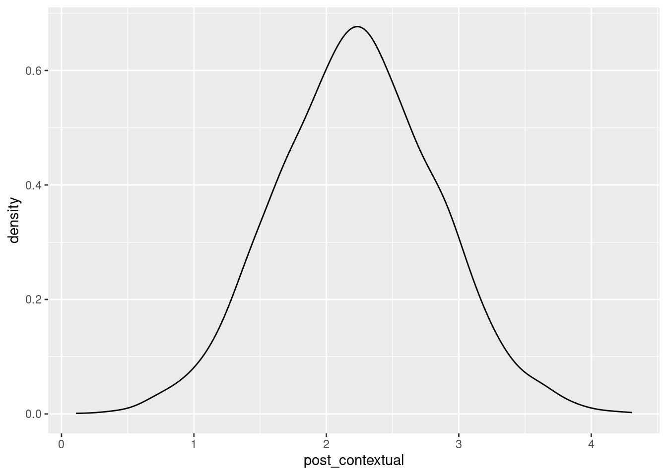
Group mean centering treating group means as latent variables
Instead of treating the group means as known, we can instead treat them as latent variables: \[X_{ij} \sim N(\mu_{Xj}, \sigma^2_X)\]
and we can set up the model with the priors:
\[\begin{align*} Y_{ij} & \sim N(\mu_j + \beta_1 (X_{ij} - \mu_{Xj}), \sigma^2) \\ X_{ij} & \sim N(\mu_{Xj}, \sigma^2_X) \\ \mu_j & \sim N(\beta_0 + \beta_2 \mu_{Xj}, \tau^2) \\ \mu_{Xj} & \sim N(0, \tau^2_X) \\ \sigma & \sim t_3(0, 10) \\ \tau & \sim t_3(0, 10) \\ \sigma_X & \sim t_3(0, 10) \\ \tau_X & \sim t_3(0, 10) \\ \beta & \sim N(0, 10) \\ \end{align*}\]
Notice that here we treat \(X\) as an outcome variable with a random intercept, just like the way we model \(Y\) when there is no predictor.
Below is the STAN code for this model:
data {
  int<lower=1> N;  // total number of observations
  int<lower=1> J;  // number of clusters
  int<lower=1, upper=J> gid[N];
  vector[N] y;  // response variable
  int<lower=1> K;  // number of population-level effects
  matrix[N, K] X;  // population-level design matrix
  int<lower=1> q;  // index of which column needs group mean centering
}
transformed data {
  int Kc = K - 1;
  matrix[N, K - 1] Xc;  // centered version of X
  vector[K - 1] means_X;  // column means of X before centering
  vector[N] xc;  // the column of X to be decomposed
  for (i in 2:K) {
    means_X[i - 1] = mean(X[, i]);
    Xc[, i - 1] = X[, i] - means_X[i - 1];
  }
  xc = Xc[, q - 1];
}
parameters {
  vector[Kc] b;  // population-level effects at level-1
  real bm;  // population-level effects at level-2
  real b0;  // intercept (with centered variables)
  real<lower=0> sigma_y;  // residual SD
  real<lower=0> tau_y;  // group-level standard deviations
  vector[J] eta_y;  // normalized group-level effects of y
  real<lower=0> sigma_x;  // residual SD
  real<lower=0> tau_x;  // group-level standard deviations
  vector[J] eta_x;  // normalized latent group means of x
}
transformed parameters {
  // group means for x
  vector[J] theta_x = tau_x * eta_x;  // group means of x
  // group-level effects
  vector[J] theta_y = b0 + tau_y * eta_y + bm * theta_x;  // group intercepts of y
  matrix[N, K - 1] Xw_c = Xc;  // copy the predictor matrix
  Xw_c[ , q - 1] = xc - theta_x[gid];  // group mean centering
}
model {
  // prior specifications
  b ~ normal(0, 10);
  bm ~ normal(0, 10);
  sigma_y ~ student_t(3, 0, 10);
  tau_y ~ student_t(3, 0, 10);
  eta_y ~ std_normal();
  sigma_x ~ student_t(3, 0, 10);
  tau_x ~ student_t(3, 0, 10);
  eta_x ~ std_normal();
  xc ~ normal(theta_x[gid], sigma_x);  // prior for lv-1 predictor
  // likelihood contribution
  y ~ normal(theta_y[gid] + Xw_c * b, sigma_y);
}
generated quantities {
  // contextual effect
  real b_contextual = bm - b[q - 1];
}
And to run it in rstan:
hsb_sdata <- with(hsb_sub,
                  list(N = nrow(hsb_sub),
                       y = MATHACH,
                       K = 2,
                       X = cbind(1, SES),
                       q = 2,
                       gid = match(ID, unique(ID)),
                       J = length(unique(ID))))
m2_stan <- stan("stan_gpc_pv.stan", data = hsb_sdata,
                chains = 2L, iter = 1000L,
                pars = c("b0", "b", "bm", "b_contextual", "sigma_y", "tau_y",
                         "sigma_x", "tau_x"))
Warning: Tail Effective Samples Size (ESS) is too low, indicating posterior variances and tail quantiles may be unreliable.
Running the chains for more iterations may help. See
https://mc-stan.org/misc/warnings.html#tail-essThe results are shown below:
print(m2_stan, pars = "lp__", include = FALSE)Inference for Stan model: anon_model.
2 chains, each with iter=1000; warmup=500; thin=1;
post-warmup draws per chain=500, total post-warmup draws=1000.
mean se_mean sd 2.5% 25% 50% 75% 97.5% n_eff Rhat
b0 12.88 0.01 0.25 12.41 12.72 12.87 13.05 13.35 1425 1.00
b[1] 2.40 0.01 0.35 1.68 2.17 2.42 2.64 3.04 839 1.00
bm 5.84 0.04 0.80 4.44 5.24 5.80 6.36 7.50 512 1.01
b_contextual 3.44 0.04 0.95 1.75 2.76 3.41 4.09 5.32 476 1.00
sigma_y 6.02 0.01 0.18 5.68 5.90 6.02 6.14 6.35 929 1.00
tau_y 1.45 0.04 0.48 0.34 1.17 1.49 1.78 2.25 176 1.00
sigma_x 0.68 0.00 0.02 0.65 0.67 0.68 0.70 0.72 1130 1.00
tau_x 0.43 0.00 0.04 0.36 0.40 0.42 0.45 0.50 374 1.01
Samples were drawn using NUTS(diag_e) at Thu Mar 21 10:34:58 2024.
For each parameter, n_eff is a crude measure of effective sample size,
and Rhat is the potential scale reduction factor on split chains (at
convergence, Rhat=1).Note that the coefficient of SES at level-2 now has a posterior mean of 5.8 with a posterior SD of 0.8, and the contextual effect has a posterior mean of 3.4 with a posterior SD of 0.95
Two-step approach using brms
Step 1: estimating measurement error in observed means
m_ses <- lmer(SES ~ (1 | ID), data = hsb_sub)
summary(m_ses)
Linear mixed model fit by REML ['lmerMod']
Formula: SES ~ (1 | ID)
Data: hsb_sub
REML criterion at convergence: 1830.9
Scaled residuals:
Min 1Q Median 3Q Max
-4.8031 -0.6035 0.0062 0.6787 2.3937
Random effects:
Groups Name Variance Std.Dev.
ID (Intercept) 0.1839 0.4289
Residual 0.4617 0.6795
Number of obs: 800, groups: ID, 160
Fixed effects:
Estimate Std. Error t value
(Intercept) 0.002775 0.041555 0.067Extract measurement estimates:
# sigma_x
sigmax <- sigma(m_ses)
# Add to data
hsb_sub <- hsb_sub %>%
  group_by(ID) %>%
  mutate(SES_gpm_se = sigmax / sqrt(n())) %>%
  ungroup()
Fit MLM, incorporating measurement error in latent group means:
m1_brm_lm <- brm(MATHACH ~ me(SES_gpm, sdx = SES_gpm_se, gr = ID) +
                   SES + (1 | ID),
                 data = hsb_sub,
                 control = list(adapt_delta = .99,
                                max_treedepth = 15))
SAMPLING FOR MODEL 'anon_model' NOW (CHAIN 1).
Chain 1:
Chain 1: Gradient evaluation took 8.8e-05 seconds
Chain 1: 1000 transitions using 10 leapfrog steps per transition would take 0.88 seconds.
Chain 1: Adjust your expectations accordingly!
Chain 1:
Chain 1:
Chain 1: Iteration:    1 / 2000 [  0%]  (Warmup)
Chain 1: Iteration:  200 / 2000 [ 10%]  (Warmup)
Chain 1: Iteration:  400 / 2000 [ 20%]  (Warmup)
Chain 1: Iteration:  600 / 2000 [ 30%]  (Warmup)
Chain 1: Iteration:  800 / 2000 [ 40%]  (Warmup)
Chain 1: Iteration: 1000 / 2000 [ 50%]  (Warmup)
Chain 1: Iteration: 1001 / 2000 [ 50%]  (Sampling)
Chain 1: Iteration: 1200 / 2000 [ 60%]  (Sampling)
Chain 1: Iteration: 1400 / 2000 [ 70%]  (Sampling)
Chain 1: Iteration: 1600 / 2000 [ 80%]  (Sampling)
Chain 1: Iteration: 1800 / 2000 [ 90%]  (Sampling)
Chain 1: Iteration: 2000 / 2000 [100%]  (Sampling)
Chain 1:
Chain 1:  Elapsed Time: 8.8 seconds (Warm-up)
Chain 1:                5.081 seconds (Sampling)
Chain 1:                13.881 seconds (Total)
Chain 1:

SAMPLING FOR MODEL 'anon_model' NOW (CHAIN 2).
Chain 2:
Chain 2: Gradient evaluation took 0.000102 seconds
Chain 2: 1000 transitions using 10 leapfrog steps per transition would take 1.02 seconds.
Chain 2: Adjust your expectations accordingly!
Chain 2:
Chain 2:
Chain 2: Iteration:    1 / 2000 [  0%]  (Warmup)
Chain 2: Iteration:  200 / 2000 [ 10%]  (Warmup)
Chain 2: Iteration:  400 / 2000 [ 20%]  (Warmup)
Chain 2: Iteration:  600 / 2000 [ 30%]  (Warmup)
Chain 2: Iteration:  800 / 2000 [ 40%]  (Warmup)
Chain 2: Iteration: 1000 / 2000 [ 50%]  (Warmup)
Chain 2: Iteration: 1001 / 2000 [ 50%]  (Sampling)
Chain 2: Iteration: 1200 / 2000 [ 60%]  (Sampling)
Chain 2: Iteration: 1400 / 2000 [ 70%]  (Sampling)
Chain 2: Iteration: 1600 / 2000 [ 80%]  (Sampling)
Chain 2: Iteration: 1800 / 2000 [ 90%]  (Sampling)
Chain 2: Iteration: 2000 / 2000 [100%]  (Sampling)
Chain 2:
Chain 2:  Elapsed Time: 7.633 seconds (Warm-up)
Chain 2:                4.678 seconds (Sampling)
Chain 2:                12.311 seconds (Total)
Chain 2:

SAMPLING FOR MODEL 'anon_model' NOW (CHAIN 3).
Chain 3:
Chain 3: Gradient evaluation took 0.000114 seconds
Chain 3: 1000 transitions using 10 leapfrog steps per transition would take 1.14 seconds.
Chain 3: Adjust your expectations accordingly!
Chain 3:
Chain 3:
Chain 3: Iteration:    1 / 2000 [  0%]  (Warmup)
Chain 3: Iteration:  200 / 2000 [ 10%]  (Warmup)
Chain 3: Iteration:  400 / 2000 [ 20%]  (Warmup)
Chain 3: Iteration:  600 / 2000 [ 30%]  (Warmup)
Chain 3: Iteration:  800 / 2000 [ 40%]  (Warmup)
Chain 3: Iteration: 1000 / 2000 [ 50%]  (Warmup)
Chain 3: Iteration: 1001 / 2000 [ 50%]  (Sampling)
Chain 3: Iteration: 1200 / 2000 [ 60%]  (Sampling)
Chain 3: Iteration: 1400 / 2000 [ 70%]  (Sampling)
Chain 3: Iteration: 1600 / 2000 [ 80%]  (Sampling)
Chain 3: Iteration: 1800 / 2000 [ 90%]  (Sampling)
Chain 3: Iteration: 2000 / 2000 [100%]  (Sampling)
Chain 3:
Chain 3:  Elapsed Time: 7.028 seconds (Warm-up)
Chain 3:                4.679 seconds (Sampling)
Chain 3:                11.707 seconds (Total)
Chain 3:

SAMPLING FOR MODEL 'anon_model' NOW (CHAIN 4).
Chain 4:
Chain 4: Gradient evaluation took 8.5e-05 seconds
Chain 4: 1000 transitions using 10 leapfrog steps per transition would take 0.85 seconds.
Chain 4: Adjust your expectations accordingly!
Chain 4:
Chain 4:
Chain 4: Iteration:    1 / 2000 [  0%]  (Warmup)
Chain 4: Iteration:  200 / 2000 [ 10%]  (Warmup)
Chain 4: Iteration:  400 / 2000 [ 20%]  (Warmup)
Chain 4: Iteration:  600 / 2000 [ 30%]  (Warmup)
Chain 4: Iteration:  800 / 2000 [ 40%]  (Warmup)
Chain 4: Iteration: 1000 / 2000 [ 50%]  (Warmup)
Chain 4: Iteration: 1001 / 2000 [ 50%]  (Sampling)
Chain 4: Iteration: 1200 / 2000 [ 60%]  (Sampling)
Chain 4: Iteration: 1400 / 2000 [ 70%]  (Sampling)
Chain 4: Iteration: 1600 / 2000 [ 80%]  (Sampling)
Chain 4: Iteration: 1800 / 2000 [ 90%]  (Sampling)
Chain 4: Iteration: 2000 / 2000 [100%]  (Sampling)
Chain 4:
Chain 4:  Elapsed Time: 10.136 seconds (Warm-up)
Chain 4:                4.666 seconds (Sampling)
Chain 4:                14.802 seconds (Total)
Chain 4:
Warning: Tail Effective Samples Size (ESS) is too low, indicating posterior variances and tail quantiles may be unreliable.
Running the chains for more iterations may help. See
https://mc-stan.org/misc/warnings.html#tail-esssummary(m1_brm_lm) Family: gaussian
Links: mu = identity; sigma = identity
Formula: MATHACH ~ me(SES_gpm, sdx = SES_gpm_se, gr = ID) + SES + (1 | ID)
Data: hsb_sub (Number of observations: 800)
Draws: 4 chains, each with iter = 2000; warmup = 1000; thin = 1;
total post-warmup draws = 4000
Multilevel Hyperparameters:
~ID (Number of levels: 160)
Estimate Est.Error l-95% CI u-95% CI Rhat Bulk_ESS Tail_ESS
sd(Intercept) 1.42 0.49 0.24 2.24 1.01 422 357
Regression Coefficients:
Estimate Est.Error l-95% CI u-95% CI Rhat
Intercept 12.88 0.26 12.35 13.39 1.00
SES 2.40 0.36 1.70 3.13 1.00
meSES_gpmsdxEQSES_gpm_segrEQID 3.46 0.94 1.65 5.32 1.00
Bulk_ESS Tail_ESS
Intercept 4037 2683
SES 3135 3081
meSES_gpmsdxEQSES_gpm_segrEQID 1600 2211
Further Distributional Parameters:
Estimate Est.Error l-95% CI u-95% CI Rhat Bulk_ESS Tail_ESS
sigma 6.01 0.17 5.69 6.35 1.00 2198 2842
Draws were sampled using sampling(NUTS). For each parameter, Bulk_ESS
and Tail_ESS are effective sample size measures, and Rhat is the potential
scale reduction factor on split chains (at convergence, Rhat = 1).With random slopes
With brms, we have
m2_brm <- brm(MATHACH ~ SES_gpm + SES_gpc + (SES_gpc | ID), data = hsb_sub,
              control = list(max_treedepth = 15, adapt_delta = .90))
SAMPLING FOR MODEL 'anon_model' NOW (CHAIN 1).
Chain 1:
Chain 1: Gradient evaluation took 8.2e-05 seconds
Chain 1: 1000 transitions using 10 leapfrog steps per transition would take 0.82 seconds.
Chain 1: Adjust your expectations accordingly!
Chain 1:
Chain 1:
Chain 1: Iteration:    1 / 2000 [  0%]  (Warmup)
Chain 1: Iteration:  200 / 2000 [ 10%]  (Warmup)
Chain 1: Iteration:  400 / 2000 [ 20%]  (Warmup)
Chain 1: Iteration:  600 / 2000 [ 30%]  (Warmup)
Chain 1: Iteration:  800 / 2000 [ 40%]  (Warmup)
Chain 1: Iteration: 1000 / 2000 [ 50%]  (Warmup)
Chain 1: Iteration: 1001 / 2000 [ 50%]  (Sampling)
Chain 1: Iteration: 1200 / 2000 [ 60%]  (Sampling)
Chain 1: Iteration: 1400 / 2000 [ 70%]  (Sampling)
Chain 1: Iteration: 1600 / 2000 [ 80%]  (Sampling)
Chain 1: Iteration: 1800 / 2000 [ 90%]  (Sampling)
Chain 1: Iteration: 2000 / 2000 [100%]  (Sampling)
Chain 1:
Chain 1:  Elapsed Time: 2.774 seconds (Warm-up)
Chain 1:                2.229 seconds (Sampling)
Chain 1:                5.003 seconds (Total)
Chain 1:

SAMPLING FOR MODEL 'anon_model' NOW (CHAIN 2).
Chain 2:
Chain 2: Gradient evaluation took 8.4e-05 seconds
Chain 2: 1000 transitions using 10 leapfrog steps per transition would take 0.84 seconds.
Chain 2: Adjust your expectations accordingly!
Chain 2:
Chain 2:
Chain 2: Iteration:    1 / 2000 [  0%]  (Warmup)
Chain 2: Iteration:  200 / 2000 [ 10%]  (Warmup)
Chain 2: Iteration:  400 / 2000 [ 20%]  (Warmup)
Chain 2: Iteration:  600 / 2000 [ 30%]  (Warmup)
Chain 2: Iteration:  800 / 2000 [ 40%]  (Warmup)
Chain 2: Iteration: 1000 / 2000 [ 50%]  (Warmup)
Chain 2: Iteration: 1001 / 2000 [ 50%]  (Sampling)
Chain 2: Iteration: 1200 / 2000 [ 60%]  (Sampling)
Chain 2: Iteration: 1400 / 2000 [ 70%]  (Sampling)
Chain 2: Iteration: 1600 / 2000 [ 80%]  (Sampling)
Chain 2: Iteration: 1800 / 2000 [ 90%]  (Sampling)
Chain 2: Iteration: 2000 / 2000 [100%]  (Sampling)
Chain 2:
Chain 2:  Elapsed Time: 2.947 seconds (Warm-up)
Chain 2:                1.222 seconds (Sampling)
Chain 2:                4.169 seconds (Total)
Chain 2:

SAMPLING FOR MODEL 'anon_model' NOW (CHAIN 3).
Chain 3:
Chain 3: Gradient evaluation took 7.8e-05 seconds
Chain 3: 1000 transitions using 10 leapfrog steps per transition would take 0.78 seconds.
Chain 3: Adjust your expectations accordingly!
Chain 3:
Chain 3:
Chain 3: Iteration:    1 / 2000 [  0%]  (Warmup)
Chain 3: Iteration:  200 / 2000 [ 10%]  (Warmup)
Chain 3: Iteration:  400 / 2000 [ 20%]  (Warmup)
Chain 3: Iteration:  600 / 2000 [ 30%]  (Warmup)
Chain 3: Iteration:  800 / 2000 [ 40%]  (Warmup)
Chain 3: Iteration: 1000 / 2000 [ 50%]  (Warmup)
Chain 3: Iteration: 1001 / 2000 [ 50%]  (Sampling)
Chain 3: Iteration: 1200 / 2000 [ 60%]  (Sampling)
Chain 3: Iteration: 1400 / 2000 [ 70%]  (Sampling)
Chain 3: Iteration: 1600 / 2000 [ 80%]  (Sampling)
Chain 3: Iteration: 1800 / 2000 [ 90%]  (Sampling)
Chain 3: Iteration: 2000 / 2000 [100%]  (Sampling)
Chain 3:
Chain 3:  Elapsed Time: 3.112 seconds (Warm-up)
Chain 3:                1.834 seconds (Sampling)
Chain 3:                4.946 seconds (Total)
Chain 3:

SAMPLING FOR MODEL 'anon_model' NOW (CHAIN 4).
Chain 4:
Chain 4: Gradient evaluation took 8e-05 seconds
Chain 4: 1000 transitions using 10 leapfrog steps per transition would take 0.8 seconds.
Chain 4: Adjust your expectations accordingly!
Chain 4:
Chain 4:
Chain 4: Iteration:    1 / 2000 [  0%]  (Warmup)
Chain 4: Iteration:  200 / 2000 [ 10%]  (Warmup)
Chain 4: Iteration:  400 / 2000 [ 20%]  (Warmup)
Chain 4: Iteration:  600 / 2000 [ 30%]  (Warmup)
Chain 4: Iteration:  800 / 2000 [ 40%]  (Warmup)
Chain 4: Iteration: 1000 / 2000 [ 50%]  (Warmup)
Chain 4: Iteration: 1001 / 2000 [ 50%]  (Sampling)
Chain 4: Iteration: 1200 / 2000 [ 60%]  (Sampling)
Chain 4: Iteration: 1400 / 2000 [ 70%]  (Sampling)
Chain 4: Iteration: 1600 / 2000 [ 80%]  (Sampling)
Chain 4: Iteration: 1800 / 2000 [ 90%]  (Sampling)
Chain 4: Iteration: 2000 / 2000 [100%]  (Sampling)
Chain 4:
Chain 4:  Elapsed Time: 3.118 seconds (Warm-up)
Chain 4:                2.253 seconds (Sampling)
Chain 4:                5.371 seconds (Total)
Chain 4: summary(m2_brm) Family: gaussian
Links: mu = identity; sigma = identity
Formula: MATHACH ~ SES_gpm + SES_gpc + (SES_gpc | ID)
Data: hsb_sub (Number of observations: 800)
Draws: 4 chains, each with iter = 2000; warmup = 1000; thin = 1;
total post-warmup draws = 4000
Multilevel Hyperparameters:
~ID (Number of levels: 160)
Estimate Est.Error l-95% CI u-95% CI Rhat Bulk_ESS
sd(Intercept) 1.71 0.42 0.76 2.44 1.00 567
sd(SES_gpc) 0.98 0.63 0.05 2.31 1.00 904
cor(Intercept,SES_gpc) 0.27 0.48 -0.81 0.96 1.00 2399
Tail_ESS
sd(Intercept) 421
sd(SES_gpc) 1718
cor(Intercept,SES_gpc) 2514
Regression Coefficients:
Estimate Est.Error l-95% CI u-95% CI Rhat Bulk_ESS Tail_ESS
Intercept 12.87 0.25 12.36 13.36 1.00 3644 3185
SES_gpm 4.66 0.49 3.67 5.58 1.00 3846 3154
SES_gpc 2.41 0.36 1.69 3.10 1.00 4540 3098
Further Distributional Parameters:
Estimate Est.Error l-95% CI u-95% CI Rhat Bulk_ESS Tail_ESS
sigma 5.97 0.18 5.63 6.32 1.00 1438 1840
Draws were sampled using sampling(NUTS). For each parameter, Bulk_ESS
and Tail_ESS are effective sample size measures, and Rhat is the potential
scale reduction factor on split chains (at convergence, Rhat = 1).Below is the STAN code for this model incorporating the unreliability of group means:
data {
  int<lower=1> N;  // total number of observations
  int<lower=1> J;  // number of clusters
  int<lower=1, upper=J> gid[N];
  vector[N] y;  // response variable
  int<lower=1> K;  // number of population-level effects
  matrix[N, K] X;  // population-level design matrix
  int<lower=1> q;  // index of which column needs group mean centering
}
transformed data {
  int Kc = K - 1;
  matrix[N, K - 1] Xc;  // centered version of X
  vector[K - 1] means_X;  // column means of X before centering
  vector[N] xc;  // the column of X to be decomposed
  for (i in 2:K) {
    means_X[i - 1] = mean(X[, i]);
    Xc[ , i - 1] = X[ , i] - means_X[i - 1];
  }
  xc = Xc[ , q - 1];
}
parameters {
  vector[Kc] b;  // population-level effects at level-1
  real bm;  // population-level effects at level-2
  real b0;  // intercept (with centered variables)
  real<lower=0> sigma_y;  // residual SD
  vector<lower=0>[2] tau_y;  // group-level standard deviations
  matrix[2, J] z_u;  // normalized group-level effects
  real<lower=0> sigma_x;  // residual SD
  real<lower=0> tau_x;  // group-level standard deviations
  cholesky_factor_corr[2] L_1; // Cholesky correlation factor of lv-2 residuals
  vector[J] eta_x;  // unscaled group-level effects
}
transformed parameters {
  // group means for x
  vector[J] theta_x = tau_x * eta_x;  // group means of x
  // group-level effects of y
  matrix[J, 2] u = (diag_pre_multiply(tau_y, L_1) * z_u)';
}
model {
  // prior specifications
  b ~ normal(0, 10);
  bm ~ normal(0, 10);
  sigma_y ~ student_t(3, 0, 10);
  tau_y ~ student_t(3, 0, 10);
  L_1 ~ lkj_corr_cholesky(2);
  // z_y ~ normal(0, 1);
  to_vector(z_u) ~ normal(0, 1);
  sigma_x ~ student_t(3, 0, 10);
  tau_x ~ student_t(3, 0, 10);
  eta_x ~ std_normal();
  xc ~ normal(theta_x[gid], sigma_x);  // prior for lv-1 predictor
  // likelihood contribution
  {
    matrix[N, K - 1] Xw_c = Xc;  // copy the predictor matrix
    vector[N] x_gpc = xc - theta_x[gid];
    vector[J] beta0 = b0 + theta_x * bm + u[ , 1];
    Xw_c[ , q - 1] = x_gpc;  // group mean centering
    y ~ normal(beta0[gid] + Xw_c * b + u[gid, 2] .* x_gpc,
               sigma_y);
  }
}
generated quantities {
  // contextual effect
  real b_contextual = bm - b[q - 1];
}
And to run it in rstan:
hsb_sdata <- with(hsb_sub,
                  list(N = nrow(hsb_sub),
                       y = MATHACH,
                       K = 2,
                       X = cbind(1, SES),
                       q = 2,
                       gid = match(ID, unique(ID)),
                       J = length(unique(ID))))
m3_stan <- stan("stan_gpc_pv_ran_slp.stan", data = hsb_sdata,
                chains = 2L, iter = 1000L,
                control = list(adapt_delta = .99, max_treedepth = 15),
                pars = c("b0", "b", "bm", "b_contextual", "sigma_y", "tau_y",
                         "sigma_x", "tau_x"))
Warning: Bulk Effective Samples Size (ESS) is too low, indicating posterior means and medians may be unreliable.
Running the chains for more iterations may help. See
https://mc-stan.org/misc/warnings.html#bulk-essWarning: Tail Effective Samples Size (ESS) is too low, indicating posterior variances and tail quantiles may be unreliable.
Running the chains for more iterations may help. See
https://mc-stan.org/misc/warnings.html#tail-essThe results are shown below:
print(m3_stan, pars = "lp__", include = FALSE)Inference for Stan model: anon_model.
2 chains, each with iter=1000; warmup=500; thin=1;
post-warmup draws per chain=500, total post-warmup draws=1000.
mean se_mean sd 2.5% 25% 50% 75% 97.5% n_eff Rhat
b0 12.88 0.01 0.24 12.42 12.72 12.89 13.04 13.36 1279 1.00
b[1] 2.39 0.01 0.34 1.72 2.15 2.39 2.62 3.03 712 1.00
bm 5.89 0.04 0.79 4.39 5.34 5.86 6.43 7.44 346 1.01
b_contextual 3.51 0.05 0.92 1.67 2.88 3.50 4.15 5.27 316 1.00
sigma_y 5.98 0.01 0.18 5.63 5.86 5.98 6.10 6.36 668 1.00
tau_y[1] 1.38 0.05 0.50 0.23 1.10 1.44 1.72 2.22 117 1.01
tau_y[2] 0.94 0.04 0.60 0.04 0.45 0.89 1.37 2.15 262 1.00
sigma_x 0.68 0.00 0.02 0.65 0.67 0.68 0.69 0.72 743 1.01
tau_x 0.43 0.00 0.04 0.36 0.40 0.43 0.45 0.51 389 1.00
Samples were drawn using NUTS(diag_e) at Thu Mar 21 10:39:15 2024.
For each parameter, n_eff is a crude measure of effective sample size,
and Rhat is the potential scale reduction factor on split chains (at
convergence, Rhat=1).Using two-step with brms
m3_brm_lm <- brm(MATHACH ~ me(SES_gpm, sdx = SES_gpm_se, gr = ID) +
                   SES +
                   (SES_gpc | ID),
                 data = hsb_sub,
                 control = list(adapt_delta = .99,
                                max_treedepth = 15))
SAMPLING FOR MODEL 'anon_model' NOW (CHAIN 1).
Chain 1:
Chain 1: Gradient evaluation took 0.000121 seconds
Chain 1: 1000 transitions using 10 leapfrog steps per transition would take 1.21 seconds.
Chain 1: Adjust your expectations accordingly!
Chain 1:
Chain 1:
Chain 1: Iteration:    1 / 2000 [  0%]  (Warmup)
Chain 1: Iteration:  200 / 2000 [ 10%]  (Warmup)
Chain 1: Iteration:  400 / 2000 [ 20%]  (Warmup)
Chain 1: Iteration:  600 / 2000 [ 30%]  (Warmup)
Chain 1: Iteration:  800 / 2000 [ 40%]  (Warmup)
Chain 1: Iteration: 1000 / 2000 [ 50%]  (Warmup)
Chain 1: Iteration: 1001 / 2000 [ 50%]  (Sampling)
Chain 1: Iteration: 1200 / 2000 [ 60%]  (Sampling)
Chain 1: Iteration: 1400 / 2000 [ 70%]  (Sampling)
Chain 1: Iteration: 1600 / 2000 [ 80%]  (Sampling)
Chain 1: Iteration: 1800 / 2000 [ 90%]  (Sampling)
Chain 1: Iteration: 2000 / 2000 [100%]  (Sampling)
Chain 1:
Chain 1:  Elapsed Time: 18.03 seconds (Warm-up)
Chain 1:                7.114 seconds (Sampling)
Chain 1:                25.144 seconds (Total)
Chain 1:

SAMPLING FOR MODEL 'anon_model' NOW (CHAIN 2).
Chain 2:
Chain 2: Gradient evaluation took 0.000125 seconds
Chain 2: 1000 transitions using 10 leapfrog steps per transition would take 1.25 seconds.
Chain 2: Adjust your expectations accordingly!
Chain 2:
Chain 2:
Chain 2: Iteration:    1 / 2000 [  0%]  (Warmup)
Chain 2: Iteration:  200 / 2000 [ 10%]  (Warmup)
Chain 2: Iteration:  400 / 2000 [ 20%]  (Warmup)
Chain 2: Iteration:  600 / 2000 [ 30%]  (Warmup)
Chain 2: Iteration:  800 / 2000 [ 40%]  (Warmup)
Chain 2: Iteration: 1000 / 2000 [ 50%]  (Warmup)
Chain 2: Iteration: 1001 / 2000 [ 50%]  (Sampling)
Chain 2: Iteration: 1200 / 2000 [ 60%]  (Sampling)
Chain 2: Iteration: 1400 / 2000 [ 70%]  (Sampling)
Chain 2: Iteration: 1600 / 2000 [ 80%]  (Sampling)
Chain 2: Iteration: 1800 / 2000 [ 90%]  (Sampling)
Chain 2: Iteration: 2000 / 2000 [100%]  (Sampling)
Chain 2:
Chain 2:  Elapsed Time: 15.703 seconds (Warm-up)
Chain 2:                7.085 seconds (Sampling)
Chain 2:                22.788 seconds (Total)
Chain 2:

SAMPLING FOR MODEL 'anon_model' NOW (CHAIN 3).
Chain 3:
Chain 3: Gradient evaluation took 0.000117 seconds
Chain 3: 1000 transitions using 10 leapfrog steps per transition would take 1.17 seconds.
Chain 3: Adjust your expectations accordingly!
Chain 3:
Chain 3:
Chain 3: Iteration:    1 / 2000 [  0%]  (Warmup)
Chain 3: Iteration:  200 / 2000 [ 10%]  (Warmup)
Chain 3: Iteration:  400 / 2000 [ 20%]  (Warmup)
Chain 3: Iteration:  600 / 2000 [ 30%]  (Warmup)
Chain 3: Iteration:  800 / 2000 [ 40%]  (Warmup)
Chain 3: Iteration: 1000 / 2000 [ 50%]  (Warmup)
Chain 3: Iteration: 1001 / 2000 [ 50%]  (Sampling)
Chain 3: Iteration: 1200 / 2000 [ 60%]  (Sampling)
Chain 3: Iteration: 1400 / 2000 [ 70%]  (Sampling)
Chain 3: Iteration: 1600 / 2000 [ 80%]  (Sampling)
Chain 3: Iteration: 1800 / 2000 [ 90%]  (Sampling)
Chain 3: Iteration: 2000 / 2000 [100%]  (Sampling)
Chain 3:
Chain 3:  Elapsed Time: 16.659 seconds (Warm-up)
Chain 3:                6.973 seconds (Sampling)
Chain 3:                23.632 seconds (Total)
Chain 3:

SAMPLING FOR MODEL 'anon_model' NOW (CHAIN 4).
Chain 4:
Chain 4: Gradient evaluation took 0.000123 seconds
Chain 4: 1000 transitions using 10 leapfrog steps per transition would take 1.23 seconds.
Chain 4: Adjust your expectations accordingly!
Chain 4:
Chain 4:
Chain 4: Iteration:    1 / 2000 [  0%]  (Warmup)
Chain 4: Iteration:  200 / 2000 [ 10%]  (Warmup)
Chain 4: Iteration:  400 / 2000 [ 20%]  (Warmup)
Chain 4: Iteration:  600 / 2000 [ 30%]  (Warmup)
Chain 4: Iteration:  800 / 2000 [ 40%]  (Warmup)
Chain 4: Iteration: 1000 / 2000 [ 50%]  (Warmup)
Chain 4: Iteration: 1001 / 2000 [ 50%]  (Sampling)
Chain 4: Iteration: 1200 / 2000 [ 60%]  (Sampling)
Chain 4: Iteration: 1400 / 2000 [ 70%]  (Sampling)
Chain 4: Iteration: 1600 / 2000 [ 80%]  (Sampling)
Chain 4: Iteration: 1800 / 2000 [ 90%]  (Sampling)
Chain 4: Iteration: 2000 / 2000 [100%]  (Sampling)
Chain 4:
Chain 4:  Elapsed Time: 20.842 seconds (Warm-up)
Chain 4:                7.022 seconds (Sampling)
Chain 4:                27.864 seconds (Total)
Chain 4: summary(m3_brm_lm) Family: gaussian
Links: mu = identity; sigma = identity
Formula: MATHACH ~ me(SES_gpm, sdx = SES_gpm_se, gr = ID) + SES + (SES_gpc | ID)
Data: hsb_sub (Number of observations: 800)
Draws: 4 chains, each with iter = 2000; warmup = 1000; thin = 1;
total post-warmup draws = 4000
Multilevel Hyperparameters:
~ID (Number of levels: 160)
Estimate Est.Error l-95% CI u-95% CI Rhat Bulk_ESS
sd(Intercept) 1.44 0.49 0.22 2.25 1.01 555
sd(SES_gpc) 1.02 0.64 0.05 2.36 1.01 788
cor(Intercept,SES_gpc) 0.24 0.50 -0.85 0.96 1.00 1995
Tail_ESS
sd(Intercept) 483
sd(SES_gpc) 1556
cor(Intercept,SES_gpc) 2180
Regression Coefficients:
Estimate Est.Error l-95% CI u-95% CI Rhat
Intercept 12.87 0.26 12.39 13.40 1.00
SES 2.39 0.38 1.65 3.13 1.00
meSES_gpmsdxEQSES_gpm_segrEQID 3.48 0.98 1.63 5.43 1.00
Bulk_ESS Tail_ESS
Intercept 6557 2848
SES 2660 2869
meSES_gpmsdxEQSES_gpm_segrEQID 1430 1924
Further Distributional Parameters:
Estimate Est.Error l-95% CI u-95% CI Rhat Bulk_ESS Tail_ESS
sigma 5.97 0.18 5.63 6.33 1.00 1971 2952
Draws were sampled using sampling(NUTS). For each parameter, Bulk_ESS
and Tail_ESS are effective sample size measures, and Rhat is the potential
scale reduction factor on split chains (at convergence, Rhat = 1).Using the Full Data
With lme4
hsb <- hsb %>% mutate(SES_gpm = ave(SES, ID), SES_gpc = SES - SES_gpm)
mfull_mer <- lmer(MATHACH ~ SES_gpm + SES_gpc + (1 | ID), data = hsb)
summary(mfull_mer)
Linear mixed model fit by REML ['lmerMod']
Formula: MATHACH ~ SES_gpm + SES_gpc + (1 | ID)
Data: hsb
REML criterion at convergence: 46568.6
Scaled residuals:
Min 1Q Median 3Q Max
-3.1666 -0.7254 0.0174 0.7558 2.9454
Random effects:
Groups Name Variance Std.Dev.
ID (Intercept) 2.693 1.641
Residual 37.019 6.084
Number of obs: 7185, groups: ID, 160
Fixed effects:
Estimate Std. Error t value
(Intercept) 12.6833 0.1494 84.91
SES_gpm 5.8662 0.3617 16.22
SES_gpc 2.1912 0.1087 20.16
Correlation of Fixed Effects:
(Intr) SES_gpm
SES_gpm 0.010
SES_gpc 0.000 0.000 With Bayesian taking into account the unreliability
hsb_sdata <- with(hsb,
                  list(N = nrow(hsb),
                       y = MATHACH,
                       K = 2,
                       X = cbind(1, SES),
                       q = 2,
                       gid = match(ID, unique(ID)),
                       J = length(unique(ID))))
# This takes about 4 minutes on my computer
m2full_stan <- stan("stan_gpc_pv.stan", data = hsb_sdata,
                    chains = 2L, iter = 1000L,
                    pars = c("b0", "b", "bm", "b_contextual",
                            "sigma_y", "tau_y", "sigma_x", "tau_x"))
Warning: Bulk Effective Samples Size (ESS) is too low, indicating posterior means and medians may be unreliable.
Running the chains for more iterations may help. See
https://mc-stan.org/misc/warnings.html#bulk-essprint(m2full_stan, pars = "lp__", include = FALSE)Inference for Stan model: anon_model.
2 chains, each with iter=1000; warmup=500; thin=1;
post-warmup draws per chain=500, total post-warmup draws=1000.
mean se_mean sd 2.5% 25% 50% 75% 97.5% n_eff Rhat
b0 12.69 0.01 0.15 12.41 12.59 12.69 12.79 12.97 282 1.01
b[1] 2.19 0.00 0.11 1.97 2.12 2.19 2.27 2.41 2211 1.00
bm 6.13 0.02 0.40 5.31 5.86 6.10 6.40 6.91 282 1.00
b_contextual 3.93 0.02 0.42 3.13 3.66 3.93 4.20 4.80 291 1.00
sigma_y 6.08 0.00 0.05 5.99 6.05 6.08 6.12 6.18 2430 1.00
tau_y 1.60 0.01 0.13 1.37 1.51 1.60 1.68 1.86 404 1.00
sigma_x 0.67 0.00 0.01 0.66 0.66 0.67 0.67 0.68 1876 1.00
tau_x 0.40 0.00 0.02 0.36 0.39 0.40 0.42 0.45 105 1.04
Samples were drawn using NUTS(diag_e) at Thu Mar 21 10:42:35 2024.
For each parameter, n_eff is a crude measure of effective sample size,
and Rhat is the potential scale reduction factor on split chains (at
convergence, Rhat=1).Note that with higher reliabilities, the results are more similar. Also, the results accounting for unreliability with the subset is much closer to the results with the full sample.
Bibliography
Enders, Craig K., and Davood Tofighi. 2007. “Centering predictor variables in cross-sectional multilevel models: A new look at an old issue.” Psychological Methods 12: 121–38. https://doi.org/10.1037/1082-989X.12.2.121.
Lüdtke, Oliver, Herbert W. Marsh, Alexander Robitzsch, Ulrich Trautwein, Tihomir Asparouhov, and Bengt Muthén. 2008. “The multilevel latent covariate model: A new, more reliable approach to group-level effects in contextual studies.” Psychological Methods 13: 203–29. https://doi.org/10.1037/a0012869.
Raudenbush, Stephen W., and Anthony S. Bryk. 2002. Hierarchical linear models: Applications and data analysis methods. 2nd ed. Thousand Oaks, CA: Sage.
Zitzmann, Steffen, Oliver Lüdtke, and Alexander Robitzsch. 2015. “A Bayesian approach to more stable estimates of group-level effects in contextual studies.” Multivariate Behavioral Research 50: 688–705. https://doi.org/10.1080/00273171.2015.1090899.