library(lavaan)This is lavaan 0.6-17
lavaan is FREE software! Please report any bugs.library(semPlot)
library(ggplot2)A power analysis and power curve example on the difference in change rate across treatment conditions with a latent change score model.
library(lavaan)This is lavaan 0.6-17
lavaan is FREE software! Please report any bugs.library(semPlot)
library(ggplot2)I was helping a colleague on a grant proposal, and they are interested in estimating the power of an intervention on some outcomes across three time points (baseline, post-intervention, follow-up). They are interested in fitting a latent change score (LCS) model. Given the complexity of the model, it’s easiest for me to run Monte Carlo simulations to estimate the power. I decided to write this down mainly because I want to have a record of simulating data with LCS, and also document the workflow for power analysis. I’d also like to write down some ideas I’ve got for more efficiently estimating power with simulations, something I’d share with my students (and was hoping they’d be interested in exploring it further, but so far they haven’t).
There are multiple ways to simulate the data. Because I eventually will be using lavaan to estimate the model parameters, I’m going to use the handy simulateData function from the lavaan package. The first thing to do is to define syntax for LCS with three time points.
Note in the following, I used the start() syntax for parameters that are free in estimation, and directly constrain parameters that are fixed in estimation. These two are the same for the purpose of simulating data, but by separating them, I can use the same syntax for both simulating data and estimating parameters.
# Syntax for LCS (based on the excellent book by Grimm et al., 2017, Chapter 16)
lcs3 <- "
# Latent true score
ly1 =~ 1 * y1
ly2 =~ 1 * y2
ly3 =~ 1 * y3
# Initial mean and variance
ly1 ~ start(0.5) * 1
ly1 ~~ start(1) * ly1
# Latent intercepts (fixed to 0 to force difference scores)
ly2 + ly3 ~ 0 * 1
# Latent disturbance (fixed to 0 to force to difference scores)
ly2 ~~ 0 * ly2
ly3 ~~ 0 * ly3
# Change score: ly_t = ly_t-1 + dy_t
ly2 ~ 1 * ly1
ly3 ~ 1 * ly2
dy2 =~ 1 * ly2
dy3 =~ 1 * ly3
# Constant change
slp =~ 1 * dy2 + 1 * dy3
slp ~ s * 1 + start(1) * 1
slp ~~ start(0.5) * slp
# Covariance between constant change and initial state
slp ~~ start(0) * ly1
# Change score intercepts
dy2 + dy3 ~ 0 * 1
# Change score disturbances (forced to constant change factor)
dy2 ~~ 0 * dy2
dy3 ~~ 0 * dy3
# Observed intercepts (fixed to 0 to force to latent true score means)
y1 + y2 + y3 ~ 0 * 1
# Observed errors
y1 ~~ ev * y1 + start(0.5) * y1
y2 ~~ ev * y2 + start(0.5) * y2
y3 ~~ ev * y3 + start(0.5) * y3
# Proportional effects
dy2 ~ beta * ly1 + start(-0.25) * ly1
dy3 ~ beta * ly2 + start(-0.25) * ly2
"
semPaths(lavaanify(lcs3))  # can be made cleaner with `semptools`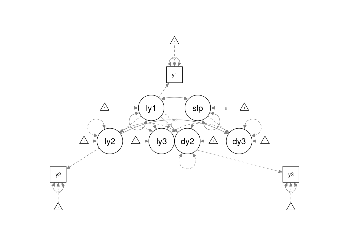
Here I simulate one data set for plotting purposes. Note that I use the empirical = TRUE argument so that the simulated data will have the exact model-implied means and covariances as the specified syntax.
sim_dat <- simulateData(lcs3, sample.nobs = 120, empirical = TRUE)
# Plot
# First, convert data to long format
reshape(data = sim_dat,
        varying = c("y1", "y2", "y3"),
        v.names = "y",
        timevar = "time",
        times = c(1, 2, 3),
        idvar = "id",
        direction = "long") |>
    # define mapping
    ggplot(aes(x = time, y = y)) +
    # add points
    geom_point(alpha = 0.3) +
    # add lines to connect the data for each person
    geom_line(aes(group = id), alpha = 0.3) +
    # add a mean trajectory
    stat_summary(fun = "mean", col = "red", linewidth = 1, geom = "line")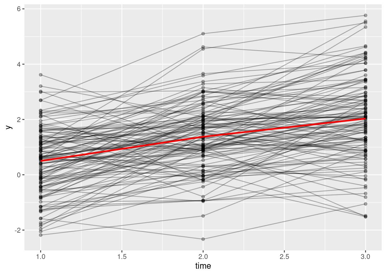
Now, I fit the model to simulated data. The fit will be perfect as I used empirical = TRUE.
lcs3_fit <- sem(lcs3, data = sim_dat)
summary(lcs3_fit)
lavaan 0.6.17 ended normally after 1 iteration
Estimator ML
Optimization method NLMINB
Number of model parameters 10
Number of equality constraints 3
Number of observations 120
Model Test User Model:
Test statistic 0.000
Degrees of freedom 2
P-value (Chi-square) 1.000
Parameter Estimates:
Standard errors Standard
Information Expected
Information saturated (h1) model Structured
Latent Variables:
Estimate Std.Err z-value P(>|z|)
ly1 =~
y1 1.000
ly2 =~
y2 1.000
ly3 =~
y3 1.000
dy2 =~
ly2 1.000
dy3 =~
ly3 1.000
slp =~
dy2 1.000
dy3 1.000
Regressions:
Estimate Std.Err z-value P(>|z|)
ly2 ~
ly1 1.000
ly3 ~
ly2 1.000
dy2 ~
ly1 (beta) -0.250 0.131 -1.915 0.055
dy3 ~
ly2 (beta) -0.250 0.131 -1.915 0.055
Covariances:
Estimate Std.Err z-value P(>|z|)
ly1 ~~
slp 0.000 0.142 0.000 1.000
Intercepts:
Estimate Std.Err z-value P(>|z|)
ly1 0.500 0.111 4.502 0.000
.ly2 0.000
.ly3 0.000
slp (s) 1.000 0.144 6.928 0.000
.dy2 0.000
.dy3 0.000
.y1 0.000
.y2 0.000
.y3 0.000
Variances:
Estimate Std.Err z-value P(>|z|)
ly1 1.000 0.195 5.140 0.000
.ly2 0.000
.ly3 0.000
slp 0.500 0.115 4.354 0.000
.dy2 0.000
.dy3 0.000
.y1 (ev) 0.500 0.065 7.746 0.000
.y2 (ev) 0.500 0.065 7.746 0.000
.y3 (ev) 0.500 0.065 7.746 0.000The previous only shows one group. In the power analysis, we’re interested in the difference in the constant change parameter (labelled s in the syntax, analogous to the slope parameter in growth curve model) across two treatment conditions. Below is the syntax for a two-group analysis.
lcs3_mg <- "
# Latent true score
ly1 =~ 1 * y1
ly2 =~ 1 * y2
ly3 =~ 1 * y3
# Initial mean and variance
ly1 ~ start(0.5) * 1
ly1 ~~ start(1) * ly1
# Latent intercepts (fixed to 0 to force difference scores)
ly2 + ly3 ~ 0 * 1
# Latent disturbance (fixed to 0 to force to difference scores)
ly2 ~~ 0 * ly2
ly3 ~~ 0 * ly3
# Change score: ly_t = ly_t-1 + dy_t
ly2 ~ 1 * ly1
ly3 ~ 1 * ly2
dy2 =~ 1 * ly2
dy3 =~ 1 * ly3
# Constant change
slp =~ 1 * dy2 + 1 * dy3
slp ~ start(c(1.112, 0.5)) * 1 + c(s1, s2) * 1
slp ~~ start(0.5) * slp
# Covariance between constant change and initial state
slp ~~ start(0) * ly1
# Change score intercepts
dy2 + dy3 ~ 0 * 1
# Change score disturbances (forced to constant change factor)
dy2 ~~ 0 * dy2
dy3 ~~ 0 * dy3
# Observed intercepts (fixed to 0 to force to latent true score means)
y1 + y2 + y3 ~ 0 * 1
# Observed errors
y1 ~~ ev * y1 + start(0.5) * y1
y2 ~~ ev * y2 + start(0.5) * y2
y3 ~~ ev * y3 + start(0.5) * y3
# Proportional effects
dy2 ~ beta * ly1 + start(-0.3) * ly1
dy3 ~ beta * ly2 + start(-0.3) * ly2
"In the syntax above, most of the parameters are constrained equal across groups, except for the constant change parameter that is hypothesized to be different across groups. This is not typical for multiple-group analysis but is common when using treatment indicator as a covariate, and may give a little bit more power when those other parameters are really equal across groups.
Plot trajectories for each treatment condition
sim_dat_mg <- simulateData(lcs3_mg, sample.nobs = c(60, 60), empirical = TRUE)Warning in lavaanify(model = model, meanstructure = meanstructure, int.ov.free = int.ov.free, : lavaan WARNING: using a single label per parameter in a multiple group
setting implies imposing equality constraints across all the groups;
If this is not intended, either remove the label(s), or use a vector
of labels (one for each group);
See the Multiple groups section in the man page of model.syntax.# Plot
reshape(data = sim_dat_mg,
varying = c("y1", "y2", "y3"),
v.names = "y",
timevar = "time",
times = c(1, 2, 3),
idvar = "id",
direction = "long") |>
ggplot(aes(x = time, y = y, color = as.factor(group))) +
geom_point(alpha = 0.1) +
# add lines to connect the data for each person
geom_line(aes(group = id), alpha = 0.05) +
# add a mean trajectory
stat_summary(fun = "mean", linewidth = 1, geom = "line",
aes(group = as.factor(group))) +
labs(color = "Group")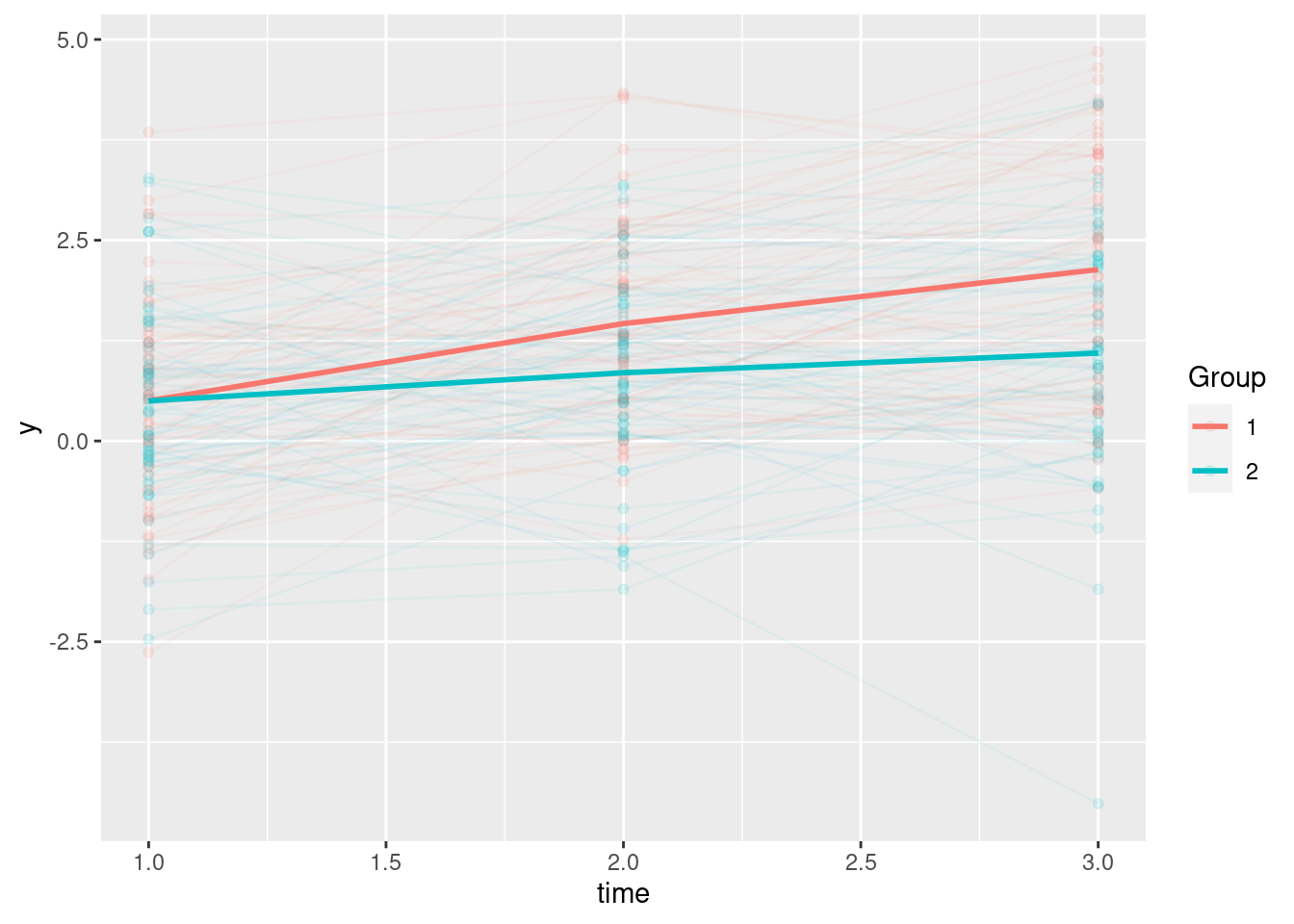
Fit to simulated data, and obtain the Wald test statistic.
lcs3_fit_mg <- sem(lcs3_mg, data = sim_dat_mg,
                   group = "group")
Warning in lavaanify(model = flat.model, constraints = constraints, varTable = DataOV, : lavaan WARNING: using a single label per parameter in a multiple group
setting implies imposing equality constraints across all the groups;
If this is not intended, either remove the label(s), or use a vector
of labels (one for each group);
See the Multiple groups section in the man page of model.syntax.summary(lcs3_fit_mg)lavaan 0.6.17 ended normally after 1 iteration
Estimator ML
Optimization method NLMINB
Number of model parameters 20
Number of equality constraints 8
Number of observations per group:
1 60
2 60
Model Test User Model:
Test statistic 0.000
Degrees of freedom 6
P-value (Chi-square) 1.000
Test statistic for each group:
1 0.000
2 0.000
Parameter Estimates:
Standard errors Standard
Information Expected
Information saturated (h1) model Structured
Group 1 [1]:
Latent Variables:
Estimate Std.Err z-value P(>|z|)
ly1 =~
y1 1.000
ly2 =~
y2 1.000
ly3 =~
y3 1.000
dy2 =~
ly2 1.000
dy3 =~
ly3 1.000
slp =~
dy2 1.000
dy3 1.000
Regressions:
Estimate Std.Err z-value P(>|z|)
ly2 ~
ly1 1.000
ly3 ~
ly2 1.000
dy2 ~
ly1 (beta) -0.300 0.142 -2.112 0.035
dy3 ~
ly2 (beta) -0.300 0.142 -2.112 0.035
Covariances:
Estimate Std.Err z-value P(>|z|)
ly1 ~~
slp 0.000 0.173 0.000 1.000
Intercepts:
Estimate Std.Err z-value P(>|z|)
ly1 0.500 0.157 3.191 0.001
.ly2 0.000
.ly3 0.000
slp (s1) 1.112 0.176 6.311 0.000
.dy2 0.000
.dy3 0.000
.y1 0.000
.y2 0.000
.y3 0.000
Variances:
Estimate Std.Err z-value P(>|z|)
ly1 1.000 0.270 3.702 0.000
.ly2 0.000
.ly3 0.000
slp 0.500 0.148 3.378 0.001
.dy2 0.000
.dy3 0.000
.y1 (ev) 0.500 0.065 7.746 0.000
.y2 (ev) 0.500 0.065 7.746 0.000
.y3 (ev) 0.500 0.065 7.746 0.000
Group 2 [2]:
Latent Variables:
Estimate Std.Err z-value P(>|z|)
ly1 =~
y1 1.000
ly2 =~
y2 1.000
ly3 =~
y3 1.000
dy2 =~
ly2 1.000
dy3 =~
ly3 1.000
slp =~
dy2 1.000
dy3 1.000
Regressions:
Estimate Std.Err z-value P(>|z|)
ly2 ~
ly1 1.000
ly3 ~
ly2 1.000
dy2 ~
ly1 (beta) -0.300 0.142 -2.112 0.035
dy3 ~
ly2 (beta) -0.300 0.142 -2.112 0.035
Covariances:
Estimate Std.Err z-value P(>|z|)
ly1 ~~
slp 0.000 0.173 0.000 1.000
Intercepts:
Estimate Std.Err z-value P(>|z|)
ly1 0.500 0.155 3.219 0.001
.ly2 0.000
.ly3 0.000
slp (s2) 0.500 0.144 3.465 0.001
.dy2 0.000
.dy3 0.000
.y1 0.000
.y2 0.000
.y3 0.000
Variances:
Estimate Std.Err z-value P(>|z|)
ly1 1.000 0.270 3.702 0.000
.ly2 0.000
.ly3 0.000
slp 0.500 0.148 3.378 0.001
.dy2 0.000
.dy3 0.000
.y1 (ev) 0.500 0.065 7.746 0.000
.y2 (ev) 0.500 0.065 7.746 0.000
.y3 (ev) 0.500 0.065 7.746 0.000lavTestWald(lcs3_fit_mg, constraints = "s1 == s2")$stat
[1] 14.89833
$df
[1] 1
$p.value
[1] 0.0001134635
$se
[1] "standard"Now, I’ll simulate 100 data sets (I used 1,000 in the actual analyses; the number here is just for a quicker illustration) and estimate the power of the Wald test, using a for loop, with a sample size of 60 per treatment condition. The difference in the constant change parameter is based on a medium effect size.
set.seed(2105)
num_sims <- 100
out <- rep(NA, num_sims)
# Design effect adjustment
clus_size <- 15
icc <- .10
deff <- 1 + (clus_size - 1) * icc
num_obs <- ceiling(60 / deff)
for (i in seq_len(num_sims)) {
    sim_dat_mg <- simulateData(lcs3_mg, sample.nobs = rep(num_obs, 2))
    lcs3_fit_mg <- sem(lcs3_mg, data = sim_dat_mg,
                   group = "group")
    out[i] <- lavTestWald(lcs3_fit_mg, constraints = "s1 == s2")$stat
}
# Simulated power
mean(pchisq(out, df = 1, lower.tail = FALSE) < .05)
[1] 0.64# Or use z test
(pow1 <- mean(pnorm(sqrt(out), lower.tail = FALSE) < .025))[1] 0.64Note that in our case, we actually had clustered data. While the more accurate way of estimating power would be to fully specify a multilevel LCS, this is difficult and would require more computational time. As a short cut, I instead use an adjustment based on the design effect, which indicates the inflation factor on the sampling variance due to clustering.
Note that the power estimate is noisy as we used a finite number of simulated data sets. We can estimate the margin of error for power, which is a proportion, as
sqrt(pow1 * (1 - pow1) / num_sims)[1] 0.048The goal here is to try to find an effect size that would give a certain level of power (e.g., 80%). While typically I would just try changing the effect size in the syntax until a get the desired level of power, a more disciplined way is to select several levels to obtain a power curve.
set.seed(2106)
num_sims <- 100
num_obs <- 60
# First, define a function for simulating data and obtaining a sample z test
sim_z <- function(nobs, s1, deff = 1 + (15 - 1) * .10, model = lcs3_mg) {
    model <- gsub("1.112", replacement = s1, x = model)
    # Simulate data (with adjusted sample size)
    sim_dat_mg <- simulateData(model, sample.nobs = rep(ceiling(nobs / deff), 2))
    # Fit model
    lcs3_fit_mg <- sem(model, data = sim_dat_mg, group = "group")
    # z statistic
    lavTestWald(lcs3_fit_mg, constraints = "s1 == s2")$stat
}
# Second, define levels of effect sizes
s1s <- c(0.5, 0.75, 1, 1.25, 1.5)
# Third, initialize output
outs <- matrix(nrow = num_sims, ncol = length(s1s))
# Fourth, simulate power with nested for loops
for (j in seq_along(s1s)) {
    for (i in seq_len(num_sims)) {
        outs[i, j] <- sim_z(nobs = num_obs, s1 = s1s[j])
    }
}
# Finally, plot power curve
pow_df <- data.frame(
    s1 = s1s,
    # Number of significant results
    nsig = apply(outs,
        MARGIN = 2,
        FUN = \(x) sum(pnorm(x, lower.tail = FALSE) < .025)
    )
)
pow_df$pow <- pow_df$nsig / num_sims
# Add number of non-significant results
pow_df$nnsig <- num_sims - pow_df$nsig
# Show power estimates
knitr::kable(pow_df)| s1 | nsig | pow | nnsig |
|---|---|---|---|
| 0.50 | 16 | 0.16 | 84 |
| 0.75 | 34 | 0.34 | 66 |
| 1.00 | 72 | 0.72 | 28 |
| 1.25 | 92 | 0.92 | 8 |
| 1.50 | 98 | 0.98 | 2 |
ggplot(pow_df, aes(x = s1, y = pow, group = 1)) +
    geom_hline(yintercept = .80) +
    geom_line() +
    geom_pointrange(aes(
        ymin = pow - 2 * sqrt(pow * (1 - pow) / num_sims),
        ymax = pow + 2 * sqrt(pow * (1 - pow) / num_sims)
    )) +
    labs(y = "power")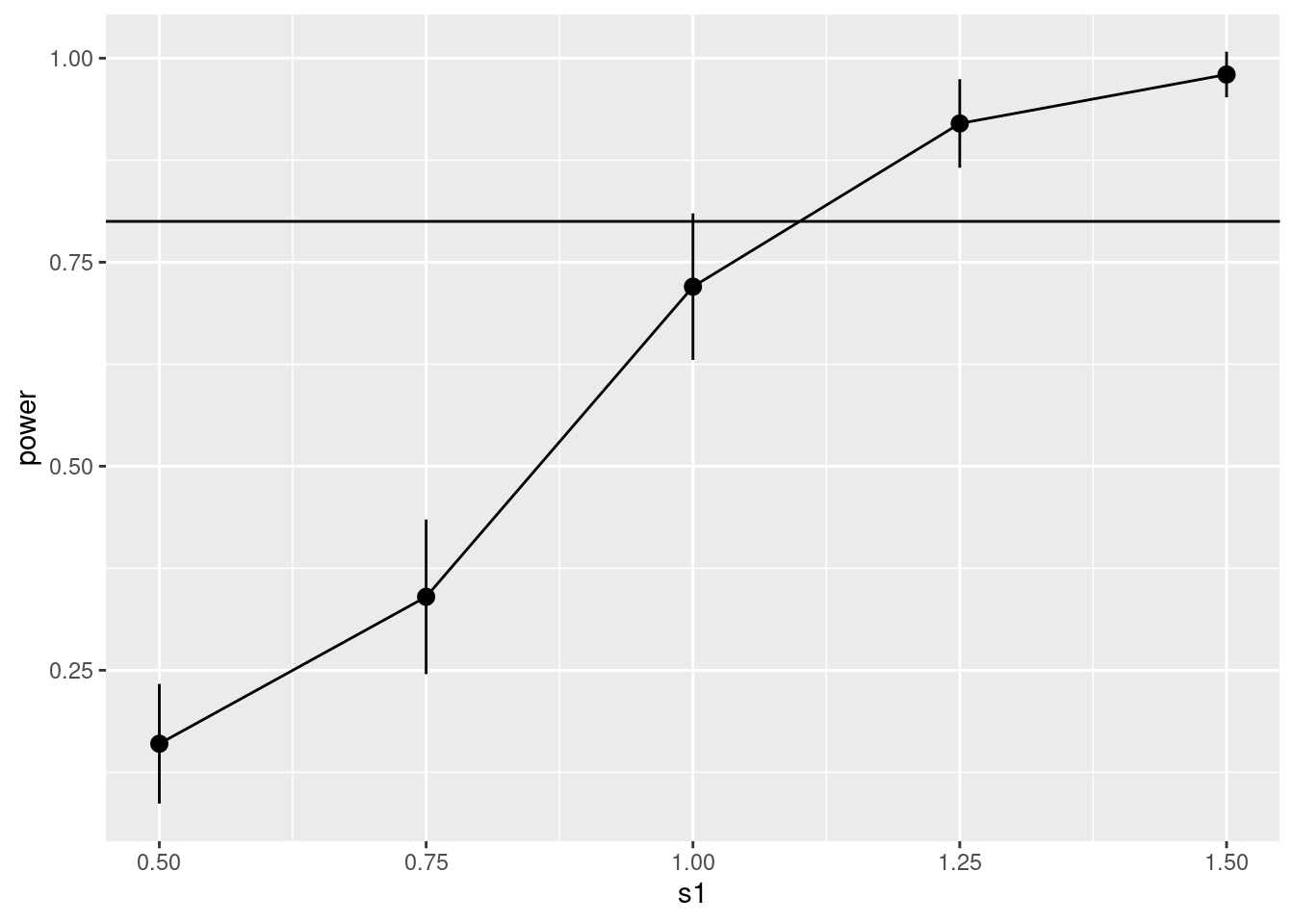
The vertical bars indicate twice the margin of error, or approximately the 95% confidence interval. This shows that we need s1 to be somewhere between 1.00 to 1.25 to achieve 80% power, but then may need to do more trial-and-error to get things more precise.
One thing I think can improve the procedure is, instead of just trial and error to find the right effect size, each time discarding information of the previous trials, we can pool re-use all the information. In simple designs like testing the mean against a null value, we know that power can be approximated as the cumulative normal distribution function of some direct function of the effect size. So we can try fitting a probit function to the power curve, and then use the model to predict the power for s1 values we haven’t tried yet. This is shown below:
ggplot(pow_df, aes(x = s1, y = pow, group = 1)) +
    geom_hline(yintercept = .80) +
    geom_smooth(
        method = "glm",
        formula = cbind(y * num_sims, (1 - y) * num_sims) ~ x,
        method.args = list(family = binomial("probit"))
    ) +
    geom_pointrange(aes(
        ymin = pow - 2 * sqrt(pow * (1 - pow) / num_sims),
        ymax = pow + 2 * sqrt(pow * (1 - pow) / num_sims)
    )) +
    labs(y = "power")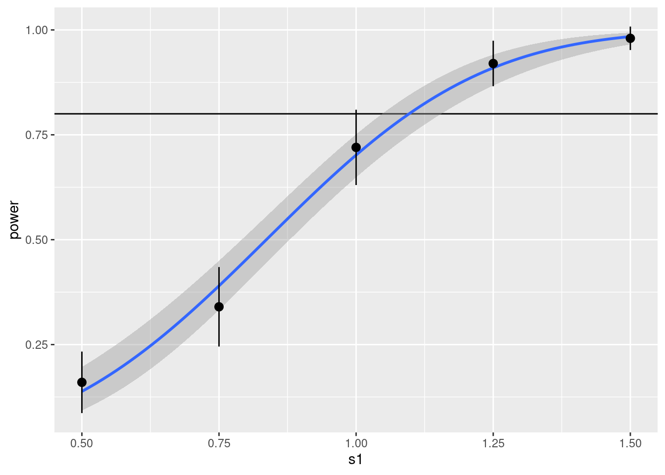
By using all data points, we get a narrower 95% confidence band around the power curve. The power curve suggests that an s1 value around 1.15 is needed to achieve 80% power.
P.S. In the above I set the nuisance parameters, such as measurement error, variance of the constant change, and the proportional effect (beta) to some predetermined values. In practice, these parameters can affect power and should be chosen carefully, and the probit approach I discussed can be used to also model power as a function of different levels of the nuisance parameters. An alternative approach is to assign Bayesian priors to those nuisance parameters to reflect the uncertainty of our knowledge, and integrate out those uncertainty when obtaining power. The latter approach is something one of my students, Winnie Tse, is currently working on (and see the hcbr package).