---
title: Confidence Intervals for Multilevel R-Squared
author: Mark Lai
date: "2022-05-12"
categories:
- Statistics
tags:
- multilevel modeling
- bootstrap
---
```{r setup, include = FALSE}
knitr::opts_chunk$set(echo = TRUE)
set.seed(2137)
```
## Load Packages
```{r load-pkg}
library(lme4)
library(MuMIn)  # for computing multilevel R-squared
library(r2mlm)  # another package for R-squared
library(bootmlm)  # for multilevel bootstrapping
library(boot)  # for bootstrap CIs
```
## An Example Multilevel Model
```{r fm1}
fm1 <- lmer(Reaction ~ Days + (Days | Subject), sleepstudy)
```
### Nakagawa-Johnson-Schielzeth $R^2$
```{r r2-fm1}
r.squaredGLMM(fm1)
```
The marginal $R^2$ considers the total variance accounted for due to the fixed effect associated with the predictors (`Days` in this example). See [Nakagawa, Johnson, & Schielzeth (2017)](https://doi.org/10.1098/rsif.2017.0213) for more information.
### Right-Sterba $R^2$
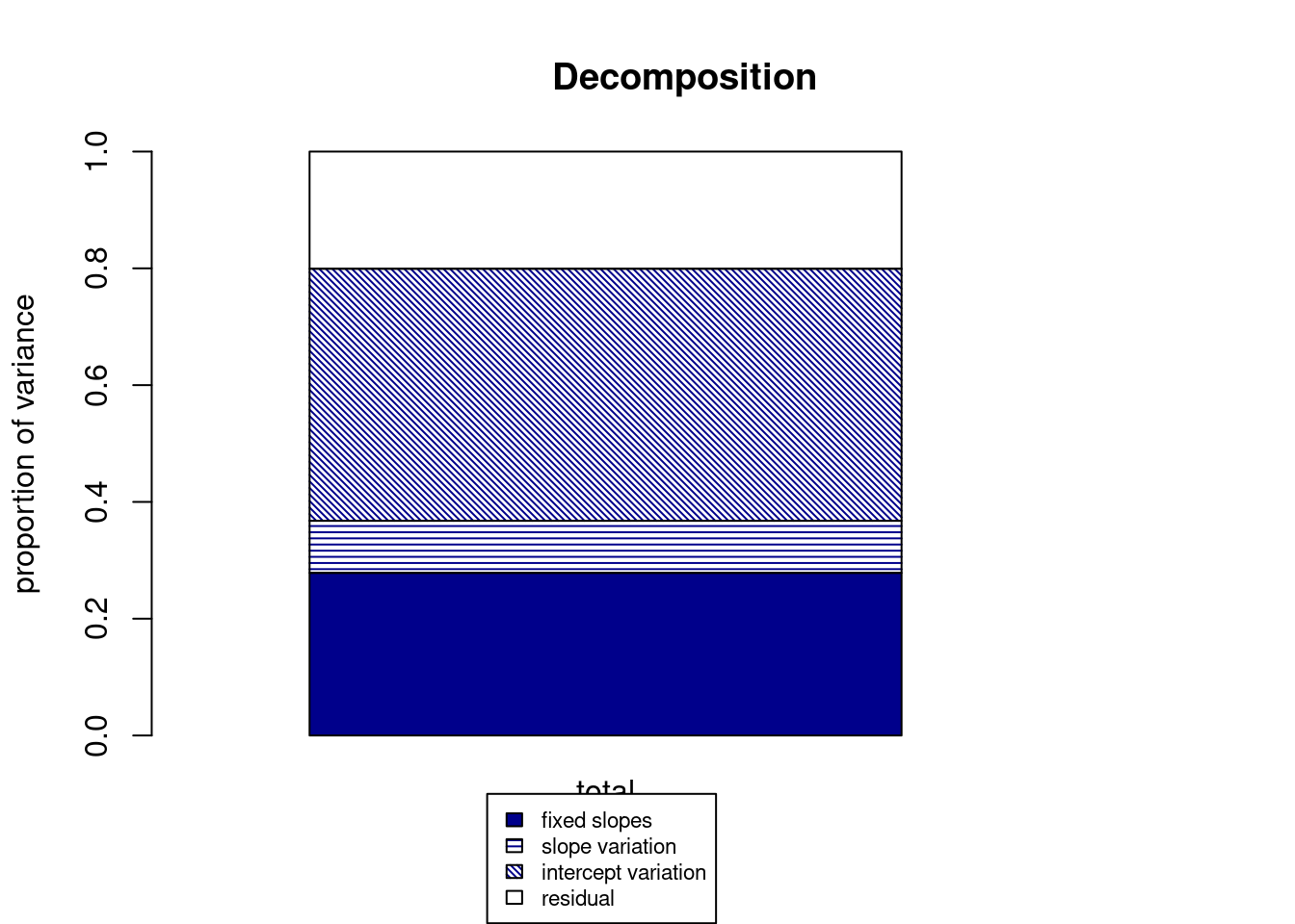
More fine-grained partitioning, as described in [Rights & Sterba (2019)](https://doi.org/10.1037/met0000184)
```{r r2mlm-fm1}
r2mlm(fm1)
```
The `fixed` part is the same as the marginal $R^2$.
## Confidence Intervals for $R^2$
Neither `MuMIn::r.squaredGLMM()` nor `r2mlm::r2mlm()` provided confidence intervals (CIs) for the $R^2$, but general guidelines for effect size reporting would suggest always reporting CIs for point estimates of effect size, just like for any point estimates in statistics. We can use multilevel bootstrapping to get CIs.
To do bootstrap, first defines an R function that gives the target $R^2$ statistics. We can do it for the marginal $R^2$:
```{r marginal_r2}
marginal_r2 <- function(object) {
  r.squaredGLMM(object)[[1]]
}
marginal_r2(fm1)
```
## Parametric Bootstrap
The `lme4::bootMer()` supports basic parametric multilevel bootstrapping
```{r boo-r2}
# This takes about 30 sec on my computer
boo01 <- bootMer(fm1, FUN = marginal_r2, nsim = 999)
boo01
```
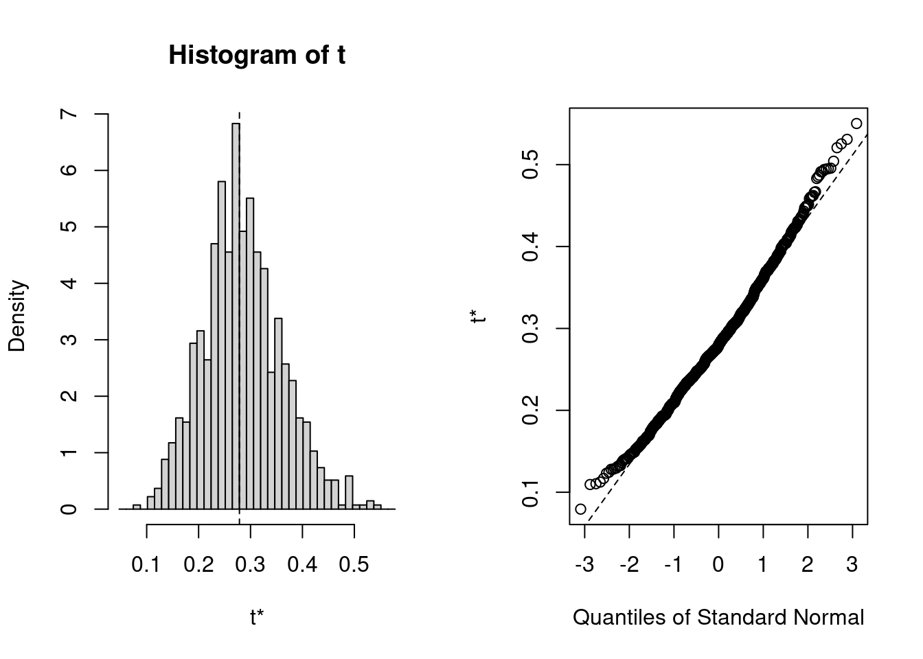
Here is the bootstrap distribution
```{r hist-boo01}
plot(boo01)
```
### Bias-corrected estimate
The above shows that the sample estimate of $R^2$ was upwardly biased. To correct for the bias, we can use the bootstrap bias-corrected estimate
```{r boot-bc-est}
2 * boo01$t0 - mean(boo01$t)
```
### Confidence intervals
You can get three types of bootstrap CIs (`"norm"`, `"basic"`, `"perc"`) with `bootMer`:
```{r boo01-ci}
boot::boot.ci(boo01, index = 1, type = c("norm", "basic", "perc"))
```
## Residual Bootstrap
The `bootmlm::bootstrap_mer()` implements the residual bootstrap, which is robust to non-normality.
```{r boo02, warning = FALSE}
# This takes about 30 sec on my computer
boo02 <- bootstrap_mer(fm1, FUN = marginal_r2, nsim = 999, type = "residual")
boo02
```
In this example, the results are similar. The boostrap bias-corrected estimate of $R^2$, and the three basic CIs, can similarly be computed as in parametric bootstrap.
### Confidence Intervals
In addition to the three CIs previously discussed, which are first-order accurate, we can also obtain CIs that are second-order accurate: (a) bias-corrected and accelerated (BCa) CI and (b) studentized CI (also called the bootstrap-$t$ CI). For (a), it requires the influence value of the $R^2$ function, whereas for (b), it requires an estimate of the sampling variance of the $R^2$ estimate.
#### Influence value
```{r emp_inf}
# Based on the group jackknife
inf_val <- bootmlm::empinf_mer(fm1, marginal_r2, index = 1)
```
#### Sampling variance with the numerical [delta method](https://en.wikipedia.org/wiki/Delta_method)
> This part is a bit more technical; skip this if you're not interested in the studentized CI.
To obtain an approximate sampling variance of the $R^2$, it would be easier to use the `r2mlm::r2mlm_manual()` function to compute $R^2$. We first write a function that computes $R^2$ using input of the fixed and random effects:
```{r deltamethod}
manual_r2 <- function(theta, data,
                      # The following are model-specific
                      wc = 2, bc = NULL, rc = 2,
                      cmc = FALSE) {
  n_wc <- length(wc)
  n_bc <- length(bc) + 1
  dim_rc <- length(rc) + 1
  n_rc <- dim_rc * (dim_rc + 1) / 2
  gam_w <- theta[seq_len(n_wc)]
  gam_b <- theta[n_wc + seq_len(n_bc)]
  tau <- matrix(NA, nrow = dim_rc, ncol = dim_rc)
  tau[lower.tri(tau, diag = TRUE)] <- theta[n_wc + n_bc + seq_len(n_rc)]
  tau2 <- t(tau)
  tau2[lower.tri(tau2)] <- tau[lower.tri(tau)]
  s2 <- tail(theta, n = 1)
  r2mlm_manual(data,
               within_covs = wc,
               between_covs = bc,
               random_covs = 2,
               gamma_w = gam_w,
               gamma_b = gam_b,
               Tau = tau2,
               sigma2 = s2,
               clustermeancentered = cmc,
               bargraph = FALSE)$R2s[1, 1]
}
theta_fm1 <- c(fixef(fm1)[2], fixef(fm1)[1],
               VarCorr(fm1)[[1]][c(1, 2, 4)], sigma(fm1)^2)
manual_r2(theta_fm1, data = fm1@frame)
```
Now computes the numerical gradient
```{r grad-fm1}
grad_fm1 <- numDeriv::grad(manual_r2, x = theta_fm1, data = fm1@frame)
```
We also need the asymptotic covariance matrix of the fixed and random effects
```{r vcov-fm1}
vcov_fixed <- vcov(fm1)
vcov_random <- vcov_vc(fm1, sd_cor = FALSE, print_names = FALSE)
vcov_fm1 <- bdiag(vcov_fixed, vcov_random)
# Need to re-arrange the first two columns
vcov_fm1 <- vcov_fm1[c(2, 1, 3:6), c(2, 1, 3:6)]
```
Now apply the multivariate delta method
```{r acov-r2}
crossprod(grad_fm1, vcov_fm1) %*% grad_fm1
```
We now need a function that computes both $R^2$ and the asymptotic sampling variance of it.
```{r marginal_r2_with_var}
marginal_r2_with_var <- function(object,
                                 wc = 2, bc = NULL, rc = 2) {
  dim_rc <- length(rc) + 1
  vc_mat <- matrix(seq_len(dim_rc^2), nrow = dim_rc, ncol = dim_rc)
  vc_index <- vc_mat[lower.tri(vc_mat, diag = TRUE)]
  theta_obj <- c(fixef(object)[wc], fixef(object)[c(1, bc)],
                 VarCorr(object)[[1]][vc_index], sigma(object)^2)
  r2 <- manual_r2(theta_obj, data = object@frame)
  grad_obj <- numDeriv::grad(manual_r2, x = theta_obj, data = object@frame)
  # Need to re-arrange the order of the fixed effects
  names_wc <- names(object@frame)[wc]
  names_bc <- c("(Intercept)", names(object@frame)[bc])
  vcov_fixed <- vcov(object)[c(names_wc, names_bc), c(names_wc, names_bc)]
  vcov_random <- vcov_vc(object, sd_cor = FALSE, print_names = FALSE)
  vcov_obj <- bdiag(vcov_fixed, vcov_random)
  v_r2 <- crossprod(grad_obj, vcov_obj) %*% grad_obj
  c(r2, as.numeric(v_r2))
}
marginal_r2_with_var(fm1)
```
#### Five Bootstrap CIs
Now, we can do bootstrap again, using the new function that computes both the estimate and the asymptotic sampling variance
```{r boo03}
# This takes quite a bit longer due to the need to compute variances
boo03 <- bootstrap_mer(fm1, FUN = marginal_r2_with_var, nsim = 999,
                       type = "residual")
boo03
```
And then obtain five types of CIs
```{r boo03-ci}
boot::boot.ci(boo03, L = inf_val)
```
## Bootstrap CI With Transformation
Given that $R^2$ is bounded, it may be more accurate to first transform the $R^2$ estimates to an unbounded scale, obtain the CIs on the transformed scale, and then back transform it to between 0 and 1. This can be done in `boot::boot.ci()` as well with the logistic transformation:
```{r boo03-ci-trans}
boot::boot.ci(boo03, L = inf_val, h = qlogis,
              # Need the derivative of the transformation
              hdot = function(x) 1 / (x - x^2),
              hinv = plogis)
```
Note that the transformation only affects the Normal, Basic, and Studentized CIs.
## Conclusion
This post demonstrates how to use multilevel bootstrapping to obtain CIs for $R^2$. The post only focuses on marginal $R^2$, but CIs for other $R^2$ measures can be similarly obtained. The studentized CI is the most complex as it requires obtaining the sampling variance of $R^2$ for each bootstrap sample. So far, to my knowledge, there has not been studies on which CI(s) perform best, so simulation studies are needed.
Further readings on multilevel bootstrap:
- [Chapter by van der Leeden et al.](https://link.springer.com/chapter/10.1007/978-0-387-73186-5_11)
- [Paper by Lai](https://doi.org/10.1080/00273171.2020.1746902)
- [Book by Davison & Hinkley](https://doi.org/10.1017/CBO9780511802843)